Posts by DavidAndolfatto:

Blockchain: what it is, what it does, and why you probably don’t need one

February 2nd, 2018

By David Andolfatto.

 

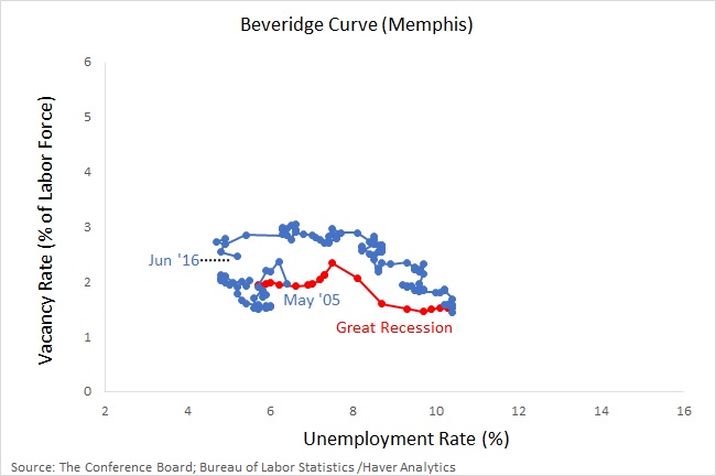
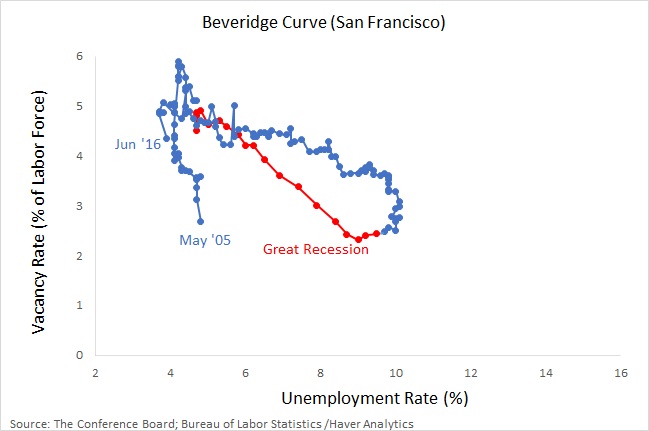
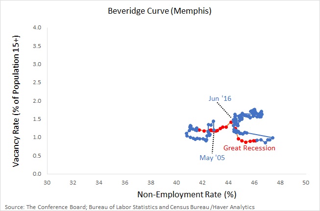
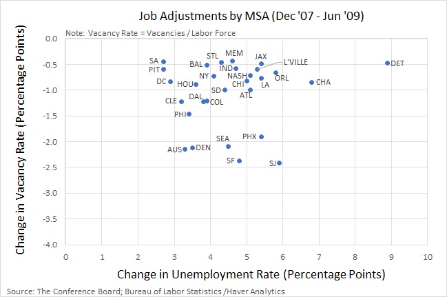
Dilbert – by Scott Adams

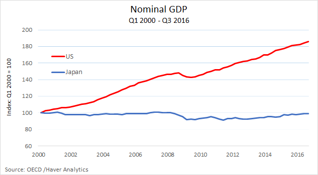
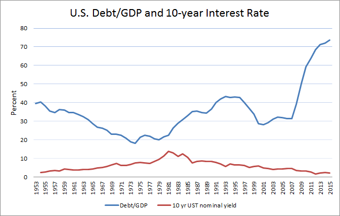
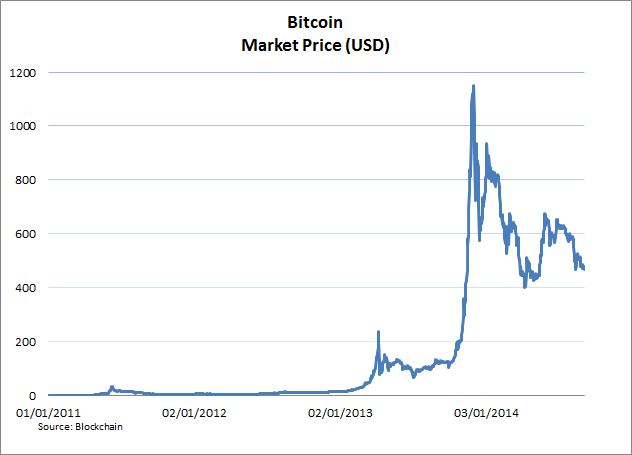
Interest in blockchain is at a fever pitch lately. This is in large part due to the eye-popping price dynamics of Bitcoin–the original bad-boy cryptocurrency–which everyone knows is powered by blockchain…whatever that is. But no matter. Given that even big players like Goldman Sachs are getting into the act (check out their super slick presentation here: Blockchain–The New Technology of Trust) maybe it’s time to figure out what all the fuss is about. What follows is based on my slide deck which I recently presented at the Olin School of Business at a Blockchain Panel (I will link up to video as soon as it becomes available)

Things are a little confusing out there I think in part because not enough care is taken in defining terms before assessing pros and cons. And when terms are defined, they sometimes include desired outcomes as a part of their definition. For example, blockchain is often described as consisting of (among other things) an immutable ledger. This is like defining a titanic to be an unsinkable ship.

So what do people mean when they bandy about the term blockchain? I recently had a chance to learn about the project from a corporate perspective as represented by Ed Corno of IBM (see IBM Blockchain), the other member of the panel I mentioned above. From Ed’s slide deck we have the following definition:

Blockchain: a shared, replicated, permissioned ledger with consensus, provenance, immutability and finality.

Well, if this is what blockchain is, then maybe I want one too! The issue I have with this definition (apart from the fact that it confounds descriptive elements with desired outcomes) is that it glosses over what I consider to be an important defining characteristic of blockchain: the consensus mechanism. Loosely speaking, there are two ways to achieve consensus. One is reputation-based (trust) and the other is game-based (trustless).

I’m not 100% sure, but I believe the corporate versions of blockchain are likely to stick to the standard model of reputation-based accounting. In this case, the efficiency gains of “blockchain” boil down to the gains associated with making databases more synchronized across trading partners, more cryptographically secure, more visible,  more complete, etc. In short, there is nothing revolutionary or radical going on here — it’s just the usual advancement of the technology and methods associated with the on-going problem of database management. Labeling the endeavor blockchain is alright, I guess. It certainly makes for good marketing!

On the other hand, game-based blockchains–like the one that power Bitcoin–are, in my view, potentially more revolutionary. But before I explain why I think this, I want to step back a bit and describe my bird’s eye view of what’s happening in this space.

A Database of Individual Action Histories

The type of information that concerns us here is not what one might label “knowledge,” say, as in the recipe for a nuclear bomb. The information in question relates more to a set of events that have happened in the past, in particular, events relating to individual actions. Consider, for example, “David washed your car two days ago.” This type of information is intrinsically useless in the sense that it is not usable in any productive manner. In addition to work histories like this, the same is true of customer service histories, delivery/receipt histories, credit histories, or any performance-related history. And yet, people value such information. It forms the bedrock of reputation and perhaps even of identity. As such, it is frequently used as a form of currency.

Why is intrinsically useless history of this form valued? A monetary theorist may tell you it’s because of a lack of commitment or a lack of trust (see Evil is the Root of All Money). If people could be relied upon to make good on their promises a priori, their track records would largely be irrelevant from an economic perspective. A good reputation is a form of capital. It is valued because it persuades creditors (believers) that more reputable agencies are more likely to make good on their promises. We keep our money in a bank not because we think bankers are angels, but because we believe the long-term franchise value of banking exceeds the short-run benefit a bank would derive from appropriating our funds. (Well, that’s the theory, at least. Admittedly, it doesn’t work perfectly.)

Note something important here. Because histories are just information, they can be created “out of thin air.” And, indeed, this is the fundamental source of the problem: people have an incentive to fabricate or counterfeit individual histories (their own and perhaps those of others) for a personal gain that comes at the expense of the community. No society can thrive, let alone survive, if its members have to worry excessively about others taking credit for their own personal contributions to the broader community. I’m writing this blog post in part (well, perhaps mainly) because I’m hoping to get credit for it.

Since humans (like bankers) are not angels, what is wanted is an honest and immutable database of histories (defined over a set of actions that are relevant for the community in question). Its purpose is to eliminate false claims of sociable behavior (acts which are tantamount to counterfeiting currency). Imagine too eliminating the frustration of discordant records. How much time is wasted in trying to settle “he said/she said” claims inside and outside of law courts? The ultimate goal, of course, is to promote fair and efficient outcomes. We may not want something like this creepy Santa Claus technology, but something similar defined over a restricted domain for a given application would be nice.

Organizing History

Let e(t) denote a set of events, or actions (relevant to the community in question), performed by an individual at date t = 1,2,3,… An individual history at date t is denoted

h(t-1) = { e(t-1), e(t-2), …, e(0) }, t = 1,2,3,…

Aggregating over individual events, we can let E(t) denote the set of individual actions at date t, and let H(t-1) denote the communal history, that is, the set of individual histories of people belonging to the community in question:

H(t-1) = { E(t-1), E(t-2), … , E(0) }, t = 1,2,3,…

Observe that E(t) can be thought of as a “block” of information (relating to a set of actions taken by members of the community at date t). If this is so, then H(t-1) consists of time-stamped blocks of information connected in sequence to form a chain of blocks. In this sense, any database consisting of a complete history of (community-relevant) events can be thought of as a “blockchain.”

Note that there are other ways of organizing history. For example, consider a cash-based economy where people are anonymous and let e(t) denote acquisitions of cash (if positive) or expenditures of cash (if negative). Then an individual’s cash balances at the beginning of date t is given by h(t-1) = e(t-1) + e(t-2) + … + e(0). This is the sense in which “money is memory.” Measuring a person’s worth by how much money they have serves as a crude summary statistic of the net contributions they’ve made to society in the past (assuming they did not steal or counterfeit the money, of course). Another way to organize history is to specify h(t-1) = { e(t-1) }. This is the “what have you done for me lately?” model of remembering favors. The possibilities are endless. But an essential component of blockchain is that it contains a complete history of all community-relevant events. (We could perhaps generalize to truncated histories if data storage is a problem.)

Database Management Systems (DBMS) and the Read/Write Privilege

Alright then, suppose that a given community (consisting of people, different divisions within a firm, different firms in a supply chain, etc.) wants to manage a chained-block of histories H(t-1) over time. How is this to be done?

Along with a specification of what is to constitute the relevant information to be contained in the database, any DBMS will have to specify parameters restricting:

1. The Read Privilege (who, what, and how);
2. The Write Privilege (who, what, and how).

That is, who gets to gets to read and write history? Is the database to be completely open, like a public library? Or will some information be held in locked vaults, accessible only with permission? And if by permission, how is this to be granted? By a trusted person, by algorithm, or some other manner? Even more important is the question of who gets to write history. As I explained earlier, the possibility for manipulation along this dimension is immense. How to guard against to attempts to fabricate history?

Historically, in “small” communities (think traditional hunter-gatherer societies) this was accomplished more or less automatically. There are no strangers in a small, isolated village and communal monitoring is relatively easy. Brave deeds and foul acts alike, unobserved by some or even most, rapidly become common knowledge. This is true even of the small communities we belong to today (at work, in clubs, families, friends, etc.). Kocherlakota (1996) labels H(t-1) in this scenario “societal memory.” I like to think of it as a virtual database of individual histories living in a distributed ledger of brains talking to each other in a P2P fashion, with additions to, and maintenance of, the shared history determined through a consensus mechanism. In this primitive DBMS, read and write privileges are largely open, the latter being subject to consensus. It all sounds so...blockchainy.

While the primitive “blockchain” described above works well enough for small societies, it doesn’t scale very well. Today, the traditional local networks of human brains have been augmented (and to some extent replaced) by a local and global networks of computers capable of communicating over the Internet. Achieving rapid consensus in a large heterogeneous community characterized by a vast flows of information is a rather daunting task.

The “solution” to this problem has largely taken the form of proprietary databases with highly restricted read privileges managed by trusted entities who are delegated the write privilege. The double-spend problem for digital money, for example, is solved by delegating the record-keeping task to a bank, located within a banking system, performing debit/credit operations on a set of proprietary ledgers connected to a central hub (a clearing agency) typically managed by a central bank.

The Problem and the Blockchain Solution

Depending on your perspective, the system that has evolved to date is either (if you are born before 1980) a great improvement over how things operated when we were young, or (if you are born post 1980) a hopelessly tangled hodgepodge of networks that have trouble communicating with each other and are intolerably vulnerable to data breaches (see figure below, courtesy Ed Corno of IBM).



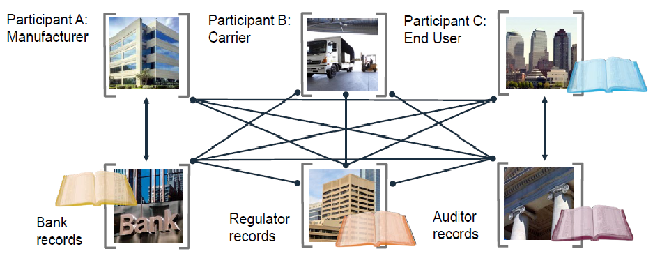
The solution to this present state of affairs is presented as blockchain (defined earlier) which Ed depicts in the following way,



Well sure, this looks like a more organized way to keep the books and clear up communication channels, though the details concerning how consensus is achieved in this system remain a little hazy to me. As I mentioned earlier, I’m guessing that it’ll be based on some reputation-based mechanism. But if this is the case, then why can’t we depict the solution in the following way?



That is, gather all the agents and agencies interacting with each other, forming them into a more organized community, but keep it based on the traditional client-server (or hub-and-spoke) model. In the center, we have the set of trusted “historians” (bankers, accountants, auditors, database managers, etc.) who are granted the write-privilege. Communications between members may be intermediated either by historians or take place in a P2P manner with the historians listening in. The database can consist of the chain-blocked sets of information (blockchain) H(t-1) described above. The parameters governing the read-privilege can be determined beforehand by the needs of the community. The database could be made completely open–which is equivalent to rendering it shared. And, of course, multiple copies of the database can be made as often as is deemed necessary.

The point I’m making is, if we’re ultimately going to depend on reputation-based consensus mechanisms, then we need no new innovation (like blockchain) to organize a database. While I’m no expert in the field of database management, it seems to me that standard protocols, for example, in the form of SQL Server 2017, can accommodate what is needed technologically and operationally (if anyone disagrees with me on this matter, please comment below).

Extending the Write Privilege: Game-Based Consensus

As explained above, extending the read-privilege is not a problem technologically. We are all free to publish our diaries online, creating a shared-distributed ledger of our innermost thoughts. Extending the write-privilege to unknown or untrusted parties, however, is an entirely different matter. Of course, this depends in part on the nature of the information to be stored. Wikipedia seems to work tolerably well. But its hard to use Wikipedia as currency. This is not the case with personal action histories. You don’t want other people writing your diary!

Well, fine, so you don’t trust “the Man.” What then? One alternative is to game the write privilege. The idea is to replace the trusted historian with a set of delegates drawn from the community (a set potentially consisting of the entire community). Next, have these delegates play a validation/consensus game designed in such a way that the equilibrium (say, Nash or some other solution concept) strategy profile chosen by each delegate at every date t = 1,2,3,… entails: (1) No tampering with recorded history H(t-1); and (2) Only true blocks E(t) are validated and appended to the ledger H(t-1).

What we have done here is replace one type of faith for another. Instead of having faith in mechanisms that rely on personal reputations, we must now trust that the mechanism governing non-cooperative play in the validation/consensus game will deliver a unique equilibrium outcome with the desired properties. I think this is in part what people mean when I hear them say “trust the math.”

Well, trusting the math is one thing. Trusting in the outcome of a non-cooperative game is quite another matter. The relevant field in economics is called mechanism design. I’m not going to get into details here, but suffice it to say, it’s not so straightforward designing mechanisms with sure-fire good properties. Ironically, mechanisms like Bitcoin will have to build up trust the old-fashioned way–through positive user experience (much the same way most of us trust our vehicles to function, even if we have little idea how an internal combustion engine works).

Of course, the same holds true for games based on reputational mechanisms. The difference is, I think, that non-cooperative consensus games are intrinsically more costly to operate than their reputational counterparts. The proof-of-work game played by Bitcoin miners, for example, is made intentionally costly (to prevent DDoS attacks) even though validating the relevant transaction information is virtually costless if left in the hands of a trusted validator. And if a lack of transparency is the problem for trusted systems, this conceptually separate issue can be dealt with by extending the read-privilege communally.

Having said this, I think that depending on the circumstances and the application, the cost associated with a game-based consensus mechanism may be worth incurring. I think we have to remain agnostic on this matter for now and see how future developments unfold.

Blockchain: Powering DAOs

If Blockchain (with non-cooperative consensus) has a comparative advantage, where might it be? To me, the clear application is in supporting Decentralized Autonomous Organizations (DAOs).  A DAO is basically a set of rules written as a computer program. Because it possesses no central authority or node, it can offer tailor-made “legal” systems unencumbered by prevailing laws and regulations, at least, insofar as transactions are limited to virtual fulfillments (e.g., debit/credit operations on a ledger).

Bitcoin is an example of a DAO, though the intermediaries that are associated with Bitcoin obviously are not. Ethereum is a platform that permits the construction of more sophisticated DAOs via the use of smart contracts. The comparative advantages of DAOs are that they permit: (1) a higher degree of anonymity;  (2) permissionless access and use; and (3) commitment to contractual terms (smart contracts).

It’s not immediately clear to me what value these comparative advantages have for registered businesses. There may be a role for legally compliant smart contracts (a tricky business for international transactions). But perhaps the potential is much more than I can presently imagine. Time will tell.

Link to my past posts on the subject of Bitcoin and Blockchain.

Comments Off on Blockchain: what it is, what it does, and why you probably don’t need one

A public finance case for keeping the Fed’s balance sheet large

February 21st, 2017

By David Andolfatto.

 



Former Fed Chair Ben Bernanke recently asked a question concerning the optimal long-run size of the Fed’s balance sheet (Should the Fed keep its balance sheet large?). Bernanke comes down on the side of “keeping the balance sheet close to its current size in the long run.” While he does not explicitly say how “size” is defined, I think it’s clear he means the size of the balance sheet measured relative to the size of the economy (say, as measured by nominal GDP). According to this measure of size, the Fed would have to grow its balance at the rate of nominal GDP growth.

In addition to the reasons reported by Bernanke, I think there’s a public finance argument to be made for keeping the Fed’s balance sheet large–at least, under certain conditions–like ensuring that the inflation mandate is met. Let me explain.

Let’s begin with a picture that most people are familiar with.



Prior to 2008, the Fed’s balance sheet was under one trillion dollars in size. Prior to 2008, it grew roughly at the same rate as the economy. Most of these assets consisted of short-term U.S. treasury securities. Most of these asset acquisitions were financed with zero-interest money (currency in circulation). Since 2008, the Fed’s balance sheet has grown to 4.5 trillion dollars. The composition of assets has moved away from short-term government debt to longer-term debt and mortgage-backed securities. Most of these asset acquisitions were financed with low-interest money (reserves).

Is 4.5 trillion a big number? Well, yes. But then, the U.S. is a big economy: the U.S. nominal GDP for 2016 is close to 19 trillion dollars. So in measuring the size of the Fed’s balance sheet, it probably makes more sense to measure size as a ratio. The following graph plots the size of the Fed’s balance sheet as a ratio of nominal GDP.



Prior to 2008, the size of the Fed’s balance relative to the economy averaged about 6%. The balance sheet size peaked in 2014 at just over 25%. Note that by this metric, the Fed’s balance sheet has been contracting since 2014.

For the record, note that the large expansion in the supply of Fed money was associated with historically low rates of inflation:



Now let’s talk about the business of banking. I like to think of a bank as an asset transformer: a bank converts relatively illiquid assets into relatively liquid liabilities. The Fed buys relatively high-yielding (but safe) securities, like U.S. treasury bonds and AAA-rated mortgage-backed securities. It pays for these acquisitions by issuing liabilities (printing money) in the form of low-interest reserves.
The Fed transforms high-interest government debt into low-interest Fed liabilities (money).

The difference between the interest the Fed earns on its assets and the interest it pays on its liabilities is an interest rate spread. Isn’t it wonderful to be able to borrow at low rates and invest at high rates? This is precisely what the Fed did with its large scale asset purchase (LSAP) program. Apart from any other effects that this intervention had on the economy, it resulted in huge profits for the Fed. Keep in mind that any profit made by the Fed is remitted to the U.S. Treasury (and thus, ultimately, to the U.S. taxpayer).

So just how much money does the Fed return to the treasury each year? I’m glad you asked, here you go:



In recent years, the Fed has been returning about $80-90 billion per year to the U.S. Treasury. While interest rates were higher in the past, the Fed’s balance sheet was much smaller–and so while the profit margin was high, the volume was low. Today the profit margin is smaller, but the balance sheet is much larger. (The distance between the red and blue lines represents the Fed’s foregone profit since it started paying interest on reserves in 2008).

What sort of rate of return does the Fed make on its portfolio? The following graph plots Fed payments to the Treasury as a ratio of the Fed’s assets.



Since the bulk of the Fed’s assets are in the form of U.S. government bonds, it should be no surprise to learn that the rate of return has generally followed the path of market interest rates downward. Still, in recent years, the annual rate of return is about 2%. Given that the Fed is presently financing these assets with cash (0%), ON RRP (0.25%) and IOER (0.50%), the profit margin is still significantly positive (though one wonders about the scope for further policy rate hikes if market rates remain low).

In light of this analysis, why are some people calling for the Fed to reduce the size of its balance sheet? Usually the concern is that a large balance sheet portends higher future inflation. But we’ve been living in a world of lowflation for many years now and we’re likely to stay there for the foreseeable future (though central banks should of course remain vigilant!). There is, in fact, some theoretical support for the notion of reducing the Fed’s policy rate (subject to the dual mandate and financial stability concerns); see, for example: The Inefficiency of Interest-Bearing National Debt.

Reducing the Fed’s balance sheet at this point in time seems like a needless loss for the U.S. taxpayer. Given that the Treasury is marketing a bond, who do you want to hold it? If the debt is held outside the Fed, the government needs some way to pay the 2% carry cost of the debt. The government will in this case have to reduce program spending, increase taxes, or increase the rate of growth of debt-issuance. Alternatively, if the Fed holds the debt, the carry cost is generally much lower. This cost-saving constitutes a net gain for the government. So why not take advantage of it?

***
P.S. I realize there are some who argue that a central bank enables big government. Since the government is too large, we need to end central banking and, in this manner, starve the beast. But this argument amounts to “let’s make the government less efficient in terms of financing their operations–that’ll force it to get smaller.” This line of argument strikes me as naïve–I’m not sure what would prevent the government from simply substituting into different methods of finance. If you want smaller G, then lobby Congress to make G smaller. But given that smaller G, it should still be financed in the most efficient manner possible. And that means following the prescription above.

Comments Off on A public finance case for keeping the Fed’s balance sheet large

Can the blockchain kill fake news?

January 25th, 2017

By David Andolfatto.

 



Not actually fake news, but good for a good laugh! 

Bloomberg View columnist Megan McArdle has an interesting article on fake news: Fact-Checking’s Infinite Regress Problem. Fake news constitutes blocks of information fabricated either wholly or in part from falsehoods to serve a political end. It is an act of commission, as opposed to a related act of omission: reporting blocks of true information chosen selectively to serve a political end.

A natural response to the problem of fake news is the emergence of fact-checkers. But on what basis are these elected or self-appointed fact-checkers to be trusted? Who will guard the guardians? The solution cannot be to appoint another layer of super-fact-checkers, since this process results in an infinite regress. Ultimately, the solution will have to reside in an answer like: “The guarded must guard the guardians.”

Fake news–or fake history, for that matter–is not something new. Every society is built on a store of publicly accessible information–a shared history–that evolves over time. But who is assigned write-privileges to this public ledger and how can they be trusted? How can we be sure that Caesar, for example, didn’t fabricate much of what is recorded in his Commentaries?

This the problem with public ledgers where everyone has a write-privilege, as we do with the Internet. But the problem is an ancient one. In small social groups, individuals sometimes spread fake news about others or themselves. Whether this information becomes part of the group’s shared history may at times depend more on its truthiness than its truthfulness. And false rumors sometimes do destroy individual reputations. A society that cannot guard against individuals freely rewriting its history for personal/political gain at the expense of the community is almost surely doomed to fail. This is not to say that societies cannot function if they rely on a shared history consisting of fake news. Indeed, they may even flourish if fake news takes the form of (say) nation-founding myths designed to promote social cohesion.

You might be wondering what any of this has to do with blockchain. Well, a blockchain is simply a shared (distributed) database (history) where the database is updated and kept secure through some communal consensus algorithm. In this piece “Why the Blockchain should be familiar to you” I argue that blockchain technology has been around for a long time. Unfortunately, there are limitations to what a distributed network of human brains talking to each other through traditional methods can accomplish as communities grow larger. But recent advancements in our brain power (computers) and communications technologies (Internet) have now made a global blockchain possible. This is exactly what Bitcoin has accomplished.

And so, as 2016 comes to a close, I put forth a whimsical question. Can blockchain (somehow) kill fake news? No, I don’t think so. Well, maybe yes, in some circumstances. (Did I mention that I’m an economist?)

The answer depends on what parts of our shared history we can expect to manage through a computer-based blockchain (and on the details of the consensus protocol). The Bitcoin blockchain appears to have solved the fake news problem for its particular application (essentially, debiting/crediting money accounts–though broader applications appear possible). Might the same principles be used to manage the database at, say, Wikipedia (see How Wikipedia Really Works: An Insider’s Wry, Brave Account)?

Ultimately, I’m afraid that the fundamental problem with fake news is not that we don’t have the technology to prevent it. The problem seems more deeply rooted in the natural (if unbecoming) human trait of preferring truthiness over truth, especially if truthiness salves where the truth might hurt. I’m not sure there’s a solution to this problem apart from trying to instill in ourselves these good Roman virtues (veritas and aequitas, in particular).

Comments Off on Can the blockchain kill fake news?

Some recent economic developments in Japan

January 12th, 2017

By David Andolfatto.

Most economic commentators seem to agree that the Japanese economy has been languishing for a very long time.  What is it about Japan that gives this impression? In this post, I suggest that while Japan certainly has its share of difficulties, the common impression of stagnant economic performance seems overstated.

For some people, almost everything you need to know about Japanese macroeconomic performance is encapsulated in this diagram:



This chart tells us that the Japanese economy produced about the same total yen value of goods and services in 2016 as it did in 2000. By way of contrast, the U.S. economy increased the total dollar value of its production by 80% over the same period of time.

But of course, our material living standards do not depend on the amount of dollars or yen an economy produces–these are just units of measurement. The diagram above would be fine to use as a comparison of macroeconomic performance if the purchasing power of dollars and yen remained stable over time. The following diagram shows that this has not been the case.



The general price level (a measure of the cost of living) rose by about 40% in the U.S. since 2000, while it declined by over 10% in Japan over the same period of time. (Note: the consumer price index behaves similarly in the U.S., but is flat for Japan over this sample period.) To put things another way, the U.S. economy has experienced inflation, while the Japanese economy has experienced deflation.

If we correct for the falling (rising) purchasing power of the dollar (yen), the first diagram above is altered as follows:



That is, since 2000, real income (nominal income adjusted for the cost of living) has risen by 35% in the U.S. and by 13% in Japan. That’s still a big gap between the two countries, though not nearly as big as the gap in nominal GDP.

But there’s something else to consider as well. The total income of a country also depends on population size. How much of the difference above is accounted for by different population growth rates? The following diagram provides the answer:



Real per capita income in both the U.S. and Japan is up about 13% and 10%, respectively, since 2000. That’s not a highly significant difference in my books, especially if we take the following into consideration. First, the recession in 2009 seems to have hit Japan much harder than the U.S. Second, in the middle of a sharp recovery dynamic from the 2009 recession, Japan suffered a severe earthquake/tsunami shock in April 2011. And third, just as the economy appeared to be recovering from this latter disaster, the Japanese government increased the consumption tax in April 2014.

There are a couple of other things I’d like to mention about the comparison above. The growth in per capita RGDP in Japan in the early 2000s largely coincided with the Koizumi era. I’ve written about this here: Another Look at the Koizumi Boom. This growth episode was driven largely by a boom in private investment. It occurred at time of declining government investment spending, a sharp reversal of the the Bank of Japan’s QE program in 2006 and, of course, continued deflation. In the U.S. in the meantime, per capita RGDP grew by almost 9% over the three years 2003-2006. That’s a pretty high rate of growth by historical standards–did people really believe this to be sustainable? (Related post here: Secular Stagnation, Then and Now).

A big concern these days has to do with productivity growth. The value of production per employed person rose at more or less the same rate in both countries from 2000-2008. But labor productivity in Japan has lagged the U.S. since then.



I suspect that some of the divergence since 2008 might be explained by composition bias. That is, in a recession, the average quality of labor rises because it is the less-skilled that are let go. We know that the employment to population ratio declined sharply in the United States in 2009 and has not yet recovered, while it declined only slightly in Japan and has since then recovered.

Here is what the picture looks like in terms of production per hour worked (data only available until 2014):



It’s interesting to compare this labor productivity dynamic with real wage rates. Here, I report two measures of real wages, each of which tell the same basic story:





Note: I’m not entirely sure whether bonuses or non-wage benefits are included in the compensation measures used to compute real wages above. Assuming that these measures are roughly comparable, the divergence between the two series is really quite striking. In Japan, in particular, while labor productivity has generally been rising, the compensation to labor has essentially flat lined. I suspect that some of the post 2014 productivity and wage dynamic for Japan may be related to the increase in the employment of low-wage workers.

Prime Minister Shinzo Abe’s policy reforms (Abenomics) are motivated by a desire to increase long-run economic growth (RGDP or per capita RGDP). It’s not clear to me how monetary policy is supposed to help in this endeavor. I do not believe that achieving the 2% inflation target will have any significant consequences for real economic growth. (And in any case, I do not think the target is even feasible given present circumstances, see: The Failure to Inflate Japan.) On the fiscal policy front, I think the April VAT increase was a mistake–I do not think Japan’s fiscal situation is as dire as many make it out to be (see previous link). The third of Abe’s arrows–structural reform–seems like the only real hope. Some of these reforms are evidently targeted at relaxing restrictions on immigrant labor. But it’s unlikely in my view that this will do much to mitigate the effects of Japan’s aging (and declining) population. And it’s not entirely clear what effect the proposed reforms will have on Japan’s stagnating real wages.

Comments Off on Some recent economic developments in Japan

Beveridge curves

October 5th, 2016

By David Andolfatto.

The Beveridge Curve refers to relationship between job vacancies and unemployment or, more generally, between business sector recruiting activity and household sector job search activity.

Theoretically, the Beveridge Curve should be negatively-sloped in V-U space. When economic prospects look promising, firms wanting to expand capacity begin to post more vacancies. For a given level of unemployment, there is an increase in labor market tightness (V/U) which makes finding a job easier for unemployed workers. The unemployment rate declines as the vacancy rate rises. The reverse holds true when economic prospects are diminished.

Empirical Beveridge Curves don’t always have the clean shape suggested by theory. Sometimes, the Beveridge Curve appears to “shift.” Beginning with Lilien (1982), there’s been an inclination to interpret shifts in the Beveridge Curve as reflecting the effects of “structural” shocks as opposed to the “cyclical” shocks that drive the normal U-V dynamic. For some recent work in this area, see my interview with Gianluca Violante here: “What Shifts the Beveridge Curve? Recruitment Effort and Financial Shocks.”

I’m not going to provide much in the way of analysis in what follows. The primary purpose of this post is just to share some data that may or may not stimulate some hypotheses. Let me begin with the BC using the JOLTS data.



Here you see the familiar cyclical pattern driven by the Great Recession and recovery. Except that the BC appears to have shifted outward. In other words, given present levels of recruiting intensity, we would have expected (based on historical experience) the unemployment rate to be significantly lower. The pattern is similar if we instead use an alternative measure of job vacancies from theHWOL (the Conference Board Help Wanted Online series).



Because the size of worker flows between employment and out-of-the-labor-force are as large as the flows between employment and unemployment, I sometimes like to use a broader measure of job search (available to work) like nonemployment (you may prefer one of the alternative measures listed here.)





This representation of the data suggests that the U.S. labor market looks a lot different today than it did prior to the Great Recession.

One of the benefits of the HWOL data is that measurements are available at the MSA level. (I also have the benefit of a great research assistant, Andew Spewak, who did all the leg work for us.) Here are few examples.









Or, in terms of nonemployment rates…









So some MSAs display a relatively stable BCs in V-U and V-N space, whereas others do not.

To get some additional sense of the heterogeneity existing at the MSA level, consider the following data, which plots the ppt change in vacancies and unemployment over the recession (2007-09) and the recovery (2009-16) for a set of selected MSAs (most of the largest ones).



Not surprisingly, the unemployment rate shot up across all the MSAs in this sample and the vacancy rate declined, though not by very much in many jurisdictions. Here is how the same set of MSAs behaved during the recovery.



Again, not a very surprising pattern, apart from the extent of the heterogeneity. If we repeat the exercise above replacing the unemployment rate with the nonemployment rate, during the recession we see,



And during the recovery,



That is, recruiting intensity in the recovery appears to be up across the board. One would expect the employment rate to be up across the board as well. But it is not. MSAs like Seattle, Denver, and Phoenix, for example, have experienced declines in the employment rate despite marked increases in their respective job vacancy rates. These differences are interesting and could have implications for (say) the relative merit of policies targeted at the aggregate vs. sectoral/regional level.

Comments Off on Beveridge curves

Jackson Hole and Fed Communication

September 24th, 2016

By Dave Andolfatto.

 

Fed chair Janet Yellen gave what I considered to be a good speech at this year’s Jackson Hole conference (see here).  Not everyone seems impressed, however. The Fed has no credibility, it seems. For example, it keeps saying it’s going to do things, like raise its policy interest rate, only to repeatedly back off. I mean, what the heck? Don’t they even know what they’re doing?

At some level, this degree of frustration is understandable. (I am less sympathetic, however, when it comes to informed journalists and market traders, who should know better.) Let me try to help ease your frustration.

The first thing to keep in mind is that monetary policy is not a precise science. Much remains to be discovered, especially since the environment (technology in particular) continues to evolve. Keep in mind that most central banks employ the services of research divisions. As Einstein is purported to have said: “If we knew what it was we were doing, it would not be called research, would it?”

That’s not to say that monetary policy makers are completely clueless. Evidence. Theory. Discussion. Debate. Experience. Wisdom. They all have a role to play in the process of formulating monetary policy. There is considerable consensus along some dimensions (e.g., keeping inflation low and stable). There is outright disagreement along other dimensions. That’s just the way it is. And it’s likely to remain this way for the foreseeable future. But in the meantime, if you live in the U.S., try to take some solace in this:

Annual Inflation Rates

Now, in terms of Yellen’s Jackson Hole speech, what are people complaining about? Well, consider this WSJ article: Yellen Cries Wolf, with the subtitle: Fed chairwoman tries to convince market that a rate rise is coming but investors aren’t listening. Of course, digging deeper into the article, the author clarifies that Yellen did not actually say that, only that she came “close” to saying it. Sigh.

The main issue here, I think, is what people expect in the way of Fed communication in terms of its economic outlook and its description/explanation of its policy rule. These are two conceptually distinct objects and are often confused.

My own personal view is that a central bank should make its policy rule clear, but that it should refrain from providing an economic outlook. So, for example, the Fed should want to make it clear that a sharp uptick in inflation would be met with a correspondingly sharp increase in its policy rate (assuming that this is an appropriate policy response). But what would be the use in having the Fed provide an outlook (a probability assessment) over future inflation? All that people need to know, really, is that the Fed is committed to keeping inflation in check. The credibility of this belief is ultimately based on reputation (see diagram above). As for forecasting the contingencies that would trigger this or that policy response, let the private forecasters do their job.

But some people want more from the Fed. They want the Fed to tell them how the economy is going to evolve in the foreseeable future (and in some cases, beyond). As if the Fed, or anyone for that matter, can actually know.

Now, if people generally appreciated the inherent difficulty in offering forecasts of this sort, I’d say that it would do no harm for a central bank to offer its economic outlook–a prognosis that would find its way in a portfolio of outlooks generated by other agencies. Market participants could then combine the information in these outlooks and, together with the Fed’s clearly stated policy rule, make their own forecast of (say) the future path of short-term interest rates.

But perhaps I’m being naive. If a central bank was to just state its policy rule and refrain from offering its outlook, it would surely be criticized for not providing the market with enough “guidance.” It is the demand for this “guidance” that compels central bankers to offer an economic outlook. Here is the outlook provided by JY (emphasized phrases my own):

Looking ahead, the FOMC expects moderate growth in real gross domestic product (GDP), additional strengthening in the labor market, and inflation rising to 2 percent over the next few years. Based on this economic outlook, the FOMC continues to anticipate that gradual increases in the federal funds rate will be appropriate over time to achieve and sustain employment and inflation near our statutory objectives. Indeed, in light of the continued solid performance of the labor market and our outlook for economic activity and inflation, I believe the case for an increase in the federal funds rate has strengthened in recent months. Of course, our decisions always depend on the degree to which incoming data continues to confirm the Committee’s outlook.

And, as ever, the economic outlook is uncertain, and so monetary policy is not on a preset course. Our ability to predict how the federal funds rate will evolve over time is quite limited because monetary policy will need to respond to whatever disturbances may buffet the economy. In addition, the level of short-term interest rates consistent with the dual mandate varies over time in response to shifts in underlying economic conditions that are often evident only in hindsight. For these reasons, the range of reasonably likely outcomes for the federal funds rate is quite wide–a point illustrated by figure 1 in your handout…The reason for the wide range is that the economy is frequently buffeted by shocks and thus rarely evolves as predicted.



And so, there you have it. Evidently, the Fed plans to raise its policy rate soon. And if it doesn’t, its credibility will be diminished. Or if it does raise rates even though conditions do not warrant it, its credibility will be again be diminished. Or, as the fan chart above demonstrates, the Fed evidently has no idea where interest rates will go. There’s no winning this game. Go back and look at the first diagram again and give it a rest.

Comments Off on Jackson Hole and Fed Communication

On the want of U.S. government debt

May 25th, 2016

By David Andolfatto.

 



 

In a recent article, Narayana Kocherlakota lays out the case for why, under present conditions, the U.S. government should be issuing more debt, using the proceeds to cut taxes, finance infrastructure spending, or both. It’s a policy that many economists, including yours truly, have been advocating for some time. And while I generally support the policy, I thought it would be useful, nevertheless, to reflect on some possible counterarguments. It’s not a slam dunk case, one way or the other, I think.

Kocherlakota does a good job explaining why a deficit-financed tax cut, or deficit-finance infrastructure spending is a good idea. I want to make it clear that the argument in favor of the policy hinges critically on the presumption that we can rely on Congress to manage the public debt over time in a responsible manner. Let’s accept this assumption, provisionally at least, in order to understand the economic argument. I will come back to the political argument later.

While the debt-to-GDP ratio (D/Y) is presently high by historical standards, it’s not unmanageable. The key is not the D/Y itself, but its trajectory over time. Clearly, D/Y cannot grow forever. And fortunately, market signals are available to monitor how the public perceives the likely path for D/Y over time. These market signals are: (1) the yields on U.S. treasury debt (at various maturities), and (2) inflation and inflation expectations. So what are these market signals telling us? The yield on U.S. treasuries is presently very low. Both inflation and inflation expectations are presently running below the Fed’s 2% target and have done so for years now. So far, so good.

The large increase in D/Y since 2008 together with plummeting yields and low inflation may seem puzzling, but it’s not really. Usually, a bad event that triggers a large increase in the public debt also triggers higher bond yields and the prospect of inflation. We can expect this to be the case in any experiment where the supply of debt increases in the face of a stable (or diminished) demand for the debt that is being issued. Think Zimbabwe or Venezuela.

But the U.S. is not Zimbabwe or Venezuela, or the Weimar Republic, for that matter. Rightly or wrongly, the U.S. treasury security is viewed by investors around the world as a safe haven asset. So when the financial crises hit in the U.S. and Europe 2008-10, investors moved en masse into U.S. treasuries (and other sovereign debt instruments viewed to be relatively safe). In short, while the supply of U.S. debt spiked up, the demand for U.S. debt increased by even more. We can infer this from the behavior of bond yields, which went down (the price of debt went up) at the time.

(1)

 



 

 

So the economic argument is simple. The U.S. government can presently borrow at essentially zero interest (more or less) even 10 years out and more. This effectively gives the fiscal authority the ability to print money (low-interest debt), so there’s no need to rely on the Fed. To the extent that domestic real economic activity is still not firing on all cylinders, why not offer temporary tax cuts to stimulate demand? Why not re-build that crumbling infrastructure, putting people to work, all financed at zero-interest? It sounds like a no-brainer.

Alright, now for a couple of counterarguments, one economic and one political.

An economic argument against temporarily increasing the public debt further (and indeed, taking measures to reduce it) could be made on the basis of the Triffin Dilemma. The economist Robert Triffin noted back in the early 1960s that world reserve currency/debt status is a double-edged sword. On the one hand, it’s great that the U.S. can just print paper that is coveted around the globe. If foreigners are willing to export their goods and services to us, expecting only paper in return, then we are extracting wealth from the rest of the world (in exchange for what ever financial service our paper is providing them).

One implication this power, if exercised, is that the world reserve currency issuer is likely to run persistent trade deficits. Triffin worried that the huge amount of U.S. currency held by foreigners exposed the U.S. to foreign risks. What might happen, for example, if foreigners suddenly decided they no longer wanted to hold USD or USTs? This could result in a sudden and dramatic change in the exchange rate, leading to domestic inflation and sharply higher bond yields.

There is also the trade-related argument that persistent trade deficits kill domestic industries and domestic employment. After all, if we can make the rest of the world work for us in exchange for paper, where is the need for us to work at all? The implied boom in domestic leisure consumption sounds good theoretically. But of course, in reality, the gains are not evenly shared. The rich gain by purchasing cheaper foreign goods. The poor are out of their jobs.

A political argument against more government debt could be made by challenging the assumption that it will be managed responsibly. This “we can’t trust future politicians to do the right thing” argument is (sadly) not without empirical merit. I am reminded of the following quip by P.J. O’Rourke,

 

“The Democrats are the party that says government will make you smarter, taller, richer, and remove the crabgrass on your lawn. The Republicans are the party that says government doesn’t work and then they get elected and prove it.”

 

I can’t help but note a certain irony here. There seems to be a strong presumption among people (Americans in particular) that the government should run its finances in the manner of a household. Economic theory is quite clear that this sentiment, however noble, is just plain wrong. The irony is that to the extent that this sentiment finds its way to being represented in Congress, it proves to be a very valuable “anchoring” device for the fiscal authority.

That is, I sometimes wonder whether US treasury debt is valued around the world the way it is precisely because it is known that Congress is impregnated with a large number of genetic “debt-ceiling” algorithms. It may not be an ideal situation from the perspective of pure economic theory, but then again, it’s not hard to think of worse scenarios.

Comments Off on On the want of U.S. government debt

Lifting Off, Sooner or Later

April 2nd, 2015

By David Andolfatto.

 

From Barron’s yesterday we have this lovely headline: Two Fed Presidents Contradict Each Other on Same Day.



From the dovish corner, Charles Evans, president of the Chicago Fed, suggested that the Fed should be patient about raising rates and not act until 2016. He said:

Given uncomfortably low inflation and an uncertain global environment, there are few benefits and significant risks to increasing interest rates prematurely. Let’s be confident that we will achieve both dual mandate goals within a reasonable period of time before taking actions that could undermine the very progress we seek.

Weighing in for the Fed hawks, Kansas City Fed president Esther George said she thought the Fed should raise rates mid-year. Her take:

This balanced approach framework supports taking steps to remove the extraordinary amount of monetary accommodation currently in place. The next phase in this process is to move the federal funds rate off its near-zero setting. While the FOMC has made no decisions about the timing of this action, I continue to support liftoff towards the middle of this year due to improvement in the labor market, expectations of firmer inflation, and the balance of risks over the medium and longer run.

I want to evaluate these two views in the context of a Taylor rule. The Taylor rule is simply a mathematical representation of how the Fed should (or will) set its policy rate in relation to the current state of the economy as measured by inflation gaps (inflation minus target inflation) and output gaps (output minus potential output). Every FOMC member presumably has a Taylor rule in mind if for no other reason than the existence of the Fed’s dual mandate (the Congressional mandate that the Fed strive to stabilize inflation and employment around some long-run targets).

A simple version of the Taylor can be written in this way:

i(t) = r* + p* + A[p(t) – p*] + B[y(t) – y*]

where i(t) is the nominal interest rate (IOER) at date t, p(t) is the inflation rate at date t, and y(t) is the (logged) real GDP at date t. The starred variables are long-run values associated with the real interest rate (r*), the inflation target (p*) and the level of “potential” GDP (y*). The parameters A and B govern how strongly the Fed reacts to deviations in the inflation target [p(t) – p*] and the output gap [y(t) – y*].

Let me start with the hawkish view (see also this presentation by Jim Bullard). According to this view, y(t) is below, but very close to y*. So, let’s just say that the output gap is zero. PCE inflation is presently around p(t) = 1%. We all know that p* = 2%, so the inflation gap is -1%. Now, we have some leeway here with respect to the parameter A, but let’s assume that the Fed responds aggressively to the inflation gap (consist with the Taylor principle) so that A=2.

Now, if we think of the long-run real rate of interest as r* = 2%, then our Taylor rule delivers i(t) = 2%. Presently, the Fed’s policy rate is i(t) = 0.25%. So, if you’re OK with these calculations, the Fed should be “lifting off” (raising its policy rate) right now. Oh, and don’t call it a “tightening.” Instead, call it a “normalization.” After all, even with i(t) = 2%, the Fed is still maintaining an accommodative stance on monetary policy because 2% is lower than the long-run target policy rate of r* + p* = 4%.

What about the doves? Because doves like to emphasize the unemployment rate, the argument of a large negative output gap is now harder for them to make (see also here). But one could reasonably make the case that the output gap–as measured, say, by the employment rate of prime-age males–is still negative, let’s say [y(t) – y*] = -1%. Let’s be generous and also assume B=1.

Now, if we continue to assume r*+p* = 4%, our dovish Taylor rule tells us that the policy rate should presently be set at  i(t) = 4% – 2% – 1% = 1%. So the recommended policy rate is lower than the hawkish case, but still significantly above 25 basis points.

Thus, if we take the historical Taylor rule as a decent policy rule (in the sense that historically, it was associated with good outcomes), then one might say that the hawks have a stronger case than the doves. Both camps should be arguing for lift-off–the only question is how much and how fast.

On the other hand, something does not seem quite right with the hawk view that things are presently close to normal and that the Fed should therefore normalize its policy rate. All we have to do is look around and observe all sorts of strange things happening. The real interest on U.S. treasuries is significantly negative, for example. Indeed, the nominal interest rate on some sovereigns is significantly negative. This does not look “normal” to a lot of people (including me). And so, maybe this is one way to rescue the dovish position. For example, one might claim that the real interest rate is now lower than it normally was, e.g., r* = 1%. (see this post by James Hamilton). If so, then this might be used to justify delaying liftoff.

Regardless of positions, everyone seems to assume that liftoff will occur sooner or later. But as Jim Bullard observed here in 2010, the promise of low rates off into the indefinite future may mean low rates (and deflation) forever. Few people seem to take this argument seriously except for, gosh, the predictions seems to be playing out (see Noah Smith’s post here). For those who hold this position, the question of liftoff becomes more like now or never, rather than sooner or later.

To conclude, we see that the contradictory views expressed by Evans and George might spring from something as basic as a disagreement on what constitutes the “natural” rate of interest r*. Further disagreement might be based on the appropriate measure of “potential” y* and on the appropriate size of the parameters A and B. There are also other concerns (like “financial stability“) that are not captured in the Taylor rule above that might lead Fed presidents to adopt different views on policy.

In the immortal words of Buffalo Springfield: “There’s something happening here, What it is ain’t exactly clear.” What this something is, its root cause, and what might be done about it seems rather elusive at the moment. And I mean elusive not in the sense that nobody knows. I mean in the sense that everyone seems to have an opinion, most of which are mutually inconsistent. It makes for interesting times, at least.

Comments Off on Lifting Off, Sooner or Later

Involuntary labor market choices?

March 29th, 2015

 

By David Andolfatto. 

 



 

My pal Roger Farmer has a lot of good ideas, but he doesn’t always use the best language to express them. In a recent post, for example, Roger asserts the following.

Participation is a voluntary choice.  Unemployment is not.

The idea that unemployment is voluntary is classical nonsense.

I do not like this language. But before I explain why I feel this way, let me first describe what I think Roger is trying to say. I think he means to say that recessions are socially inefficient outcomes, manifesting themselves primarily in the form elevated levels of unemployment and not in low participation rates. The unemployed are people without good-paying jobs, but looking for good-paying jobs. Good-paying jobs are relatively scarce in a recession (especially for individuals with lower skill sets–the young, those without advanced education, etc.) If you were to interview the unemployed during a deep recession and ask them how they’re feeling, most of them would are likely to reply that they are not doing well relative to when they were employed. Economists (classical or otherwise) would say that recessions are welfare-reducing events for most people. The “classical” idea that there is little a government can or should do to help society in a deep recession is nonsense.

I think this probably captures Roger’s view fairly well. Notice, however, that nowhere did I employ the adjectives “voluntary” or “involuntary” to describe labor market outcomes. I did not because these labels are not useful (which I why we do not see these terms used in the labor literature). Indeed, want to go a step further and argue that the use of these labels might be worse than useless. Now let me explain why I feel this way.

Let’s start with some things I think we can all agree on. First, people are endowed with some time, T. Second, there are competing uses for this time. Let me assume, for simplicity, that there are three uses of time: work (e), search (u), and leisure (n). Think of “work” as time devoted toward producing marketable goods and services, “unemployment” as searching for work, and “leisure” as producing non-marketable goods and services. Third, we can all agree that we face a time constraint: e + u + n = T.

Now, suppose for simplicity that T is indivisible: it must be allocated to one and only one of the three available time-use categories (the allocation can, however, change over calendar time). In this case, a standard labor force survey (LFS) will record e = T as employment, u = T as unemployment, and n = T as nonparticipation (or not-in-the-labor-force, NILF). [Note: the LFS never asks people whether they are unemployed or not. It asks whether they have done any paid work in the previous 4 weeks and if they have not, it then asks a series a questions relating to job search activities. If they report no job search activity, they are then classified as NILF.]

Now, Roger seems to be saying that people have a choice to make when it comes to allocating their time to either work (e = T) or leisure (n = T), but that they have no choice in determining time spent unemployed (u = T). Moreover, the idea that people may choose u = T constitutes “classical nonsense.” But is this really what he means to say?

Let’s start with a basic neoclassical model. In this abstraction, individuals and firms meet in a centralized market place and individuals are assumed to know where to find the best price for their labor. Put another way, there is absolutely no reason to devote precious time to searching for work. To put it yet another way, the neoclassical model was never designed to explain unemployment–it was designed to explain employment (and non-employment). And so, in the neoclassical model, where search is not necessary, individuals rationally choose u = 0.

Now, you may think this is a silly abstraction and that you want to impose (involuntarily) the state u = T on some individuals. But why? Unemployment is not idleness. Unemployment (at least the way the LFS defines it) constitutes the activity of searching for work–it is a form of investment (that hopefully pays off in a better job opportunity in a world where finding jobs is costly). Individuals not working and not searching are counted as out of the labor force (and even these people may not be “idle” because they might be doing housework or schoolwork, etc.).

So back to our neoclassical model. Since there is no unemployment, the time-allocation problem boils down to choosing between work and leisure. Depending on idiosyncratic considerations (the price of one’s specific labor, wealth position, the opportunities for home production, schooling, etc.), some individuals choose work and others choose leisure. In the neoclassical model, these idiosyncratic “shocks” are largely beyond an individual’s control. If the demand for your labor declines, it will cause the market price of your labor to fall. You will not like that. The shock is involuntary. BUT, you still get to choose whether to work at that (or some other) lower wage, or exit the labor force. To take another example, suppose that a source of non-labor income suddenly vanishes (involuntary). You may now be compelled to take that lousy paying job. Should we label this outcome “involuntary employment?” If so, then what next? Involuntary saving? (oops). Are all choices to be considered “involuntary?”

This is not the way we (as economists) want to go, in my opinion. In my view, it makes more sense to view choices as voluntary and responsive to the incentives imposed on individuals by the economic environment. If we want to view anything as “involuntary,” it would be exogenous changes to the environment that reduce material living standards.  If circumstances change for the better, welfare increases. If they change for the worse, welfare declines. In either case, people can be expected to allocate their scarce time toward the activities that promise the highest expected payoff. What room is there left for the “voluntary/involuntary” distinction? None, in my view.

Let’s stick with the neoclassical model for a bit longer, but tweak it the way I did here to permit multiple equilibria. Now, this is right up Roger’s alley. All individual choices here are rational and “voluntary.”  But this doesn’t mean that the economy operates perfectly all the time. Indeed, the economy might get stuck in a bad equilibrium, where employment is low, non-employment is high (and unemployment is still zero). What would Roger suggest here in the way of labels? Is this a model of involuntary leisure?  How does this label help us understand anything? I argue that it does not.

Alright, so I don’t find the “involuntary leisure” label useful. So what? Well, I don’t want to make too much of this, but I think such labels can lead to muddled thinking. The label “involuntary” suggests that individuals may not respond to incentives (after all, they evidently have no choice in the matter). I think it’s better, from the perspective of designing a proper intervention, to view the individual’s circumstances as beyond their control, but to respect the fact that they are likely to respond to altered incentives. We are economists, after all — why would we not interpret the world this way? People demonstrably do respond to incentives!

I could go on and talk at length about abandoning the neoclassical assumption of centralized labor markets and replacing this construct with a decentralized search market. There is a big literature on labor market search and I’m not about to review it here. If you’re interested, read my Palgrave Dictionary entry on the subject here. Suffice it to say that I find no value in interpreting an individual’s state of unemployment as “involuntary” either. There are all sorts of jobs out there and I think people rationally turn “ill-suited” job opportunities down to search for better matches (the way I did, when I lost my construction job in the 1981 recession). Sometimes, people get “discouraged” and exit the labor force. These are all choices that people make relative to the circumstances they find themselves in. If we want to design programs to help the unfortunate (some of whom are employed or out of the labor force), then we want to design a system that respects incentives.

What’s that you say? You don’t believe that incentives matter? Not for the unemployed? This is what I call nonsense. Consider, for example, the well-known “spike” in unemployment exit rates at the point of unemployment benefit exhaustion (see David Card here: “In Austria, the exit rate from registered unemployment rises by over 200% at the expiration of benefits…”). We see clear evidence that the unemployed do respond to incentives–they do have choices, especially in an economy with so many competing uses for time. Interpreting unemployment as “voluntary” does not mean that we are to have no compassion for the the unemployed. We feel bad for anyone (employed or out of the labor force too) who face terrible circumstances beyond their control. What it means is that we should measure economic welfare based on consumption (material living standards), not time allocation choices. It means is that we understand and respect the fact that people make choices based on the incentives they face. It means that a well-designed policy should respect these incentives.

Let me sum up here. Commentators attach the label “involuntary” to unemployment to emphasize the fact that the unemployed are not typically happy with their circumstances. Fine. But then can the same not be said of many people who find themselves “involuntarily” employed (the working poor, for example) or “involuntarily” out of the labor force (looking after a sick relative, for example)? If so, then how can one unequivocally proclaim that “participation is a voluntary choice, unemployment is not?” It makes no sense to me. I want to ask Roger to stop using bad language.

Comments Off on Involuntary labor market choices?

Who’s Afraid of Deflation?

September 25th, 2014

 

 

By David Andolfatto.



Everyone knows that deflation is bad. Bad, bad, bad. Why is it bad? Well, we learned it in school. We learned it from the pundits on the news. The Great Depression. Japan. What, are you crazy? It’s bad. Here, let Ed Castranova explain it to you (Wildcat Currency, pp.160-61):

Deflation means that all prices are falling and the currency is gaining in value. Why is this a disaster? … If you hold paper money and see that it is actually gaining in value, it may occur to you that you can increase your purchasing power–make a profit–by not spending it…But if many people hold on to their money, this can dramatically reduce real economic activity and growth…

In this post, I want to report some data that may lead people to question this common narrative. Note, I am not saying that there is no element of truth in the interpretation (maybe there is, maybe there isn’t). And I do not want to question the likely bad effects that come about owing to a large unexpected deflation (or inflation).  What I want to question is whether a period of prolonged moderate (and presumably expected) deflation is necessarily associated with periods of depressed economic activity. Most people certainly seem to think so. But why?

The first example I want to show you is for the postbellum United States (source):



Following the end of the U.S. civil war, the price-level (GDP deflator) fell steadily for 35 years. In 1900, it was close to 50% of its 1865 value. In the meantime, real per capita GDP grew by 85%. That’s an average annual growth rate of about 1.8% in real per capita income. The average annual rate of deflation was about 2%. I wonder how many people are aware of this “disaster?”

O.K., well maybe that was just long ago. Sure. Let’s take a look at some more recent data from the United States, the United Kingdom, and Japan. The sample period begins in 2009 (the trough of the Great Recession) and ends in late 2013. Here is what the price level dynamic looks like since 2009:



Over this five year period, the price level is up about 7% in the United States and about 11% in the United Kingdom. As for Japan, well, we all know about the Japanese deflation problem. Over the same period of time, the price level in Japan fell by almost 7%.

Now, I want you to try to guess what the recovery dynamic–measured in real per capita GDP–looks like for each of these countries. Surely, the U.K. must be performing relatively well, Japan relatively poorly, and the U.S. somewhere in the middle?

You would be correct in supposing that the U.S. is somewhere in the middle:



But you would have mixed up the U.K. with Japan. Since the trough of the past recession, Japanese real per capita GDP is up 15% (as of the end of 2013)–roughly 3% annual growth rate. Is deflation really so bad? Maybe the Japanese would like the U.K. style inflation instead? I don’t get it.

I have some more evidence to contradict the notion of deflation discouraging spending (transactions). The evidence pertains to Bitcoin and the data is available here:Blockchain.

Many people are aware of the massive increase in the purchasing power of Bitcoin over the past couple of years (i.e., a massive deflationary episode). As is well-known, the protocol is designed such that the total supply of bitcoins will never exceed 21M units. In the meantime, this virtual currency and payment system continues to see its popularity and use grow.



One might think that given the prospect of continued long run deflation–i.e, price appreciation (it’s hard to believe that holders of bitcoin are thinking anything else)–that people would generally be induced to hoard and not spend their bitcoins. And yet, available data seems to suggest that this may not be the case:



Maybe deflation is not so bad after all?  Let’s hope so, because we may all have to start getting used to the idea!

Comments Off on Who’s Afraid of Deflation?

Excess reserves and inflation risk: A model

September 1st, 2014

 

By David Andolfatto.

I should have known better than to reason from accounting identities. But that’s basically what I did in my last post and Nick Rowe called me out on it here. So I decided to go back and think through the exercise I had in mind using a simple model economy.
Consider a simple OLG model, with 2-period-lived agents. The young are endowed with output, y. Let N denote the number of young agents (normalize N=1). The young care only about consumption when they are old (hence, they save all their income y when young). Agents are risk-averse, with expected utility function E[u(c)]. There is a storage technology. If a young agent saves k units of output when young, he gets x*f(k) units of output in the next period, where x is a productivity parameter and f(.) is an increasing and strictly concave function (there are diminishing returns to capital accumulation). Assume that capital depreciates fully after it is used in production.
If x*f'(y) > 1, the economy is dynamically efficient. If x*f'(y) < 1, the economy is dynamically inefficient (and there is a welfare-enhancing role for government debt).
Now, imagine that there are two such economies, each in a separate location. Moreover, suppose that a known fraction 0 < s < 1 of young agents from each location migrate to the “foreign” location. The identity of who migrates is not known beforehand, so there is idiosyncratic risk, but no aggregate risk.
Next, assume that there are two other assets, money and bonds, both issued by the government supply (and endowed to the initial old). Let M be the supply of money, and let B denote the supply of bonds. Let D denote the total supply of nominal government debt:
[1] D = M + B
Money is a perpetuity that pays zero nominal interest. Bonds are one-period risk-free claims to money. (Once the bonds pay off, the government just re-issues a new bond offering B to suck cash back out of the system.) Assume that the government keeps D constant maintains a fixed bond/money ratio z = B/M, so that [1] can be written as:
[2] D = (1+z)*M
In what follows, I will keep D constant throughout and consider the effect of changing z (once and for all). Note, I am comparing steady-states here. Also, since D and M remain constant over time, and since there is no real growth in this economy, I anticipate that the steady state inflation rate will be equal to zero.
Let R denote the gross nominal interest rate (also the real interest rate, since inflation is zero). Assume that the government finances the carrying cost of its interest-bearing debt with a lump-sum tax,
[3] T = (R-1)*B
The difference between money and bonds is that bonds (or intermediated claims to bonds) cannot be transported across locations. Only money is transportable. The effect of this assumption is to impose a cash-in-advance constraint (CIA) on the young agents who move across locations. (Hence, we can interpret the relocation shock as an idiosyncratic liquidity shock).
Young agents are confronted with a portfolio allocation problem. Let P denote the price level. Since the young do not consume, they save their entire nominal income, P*y. Savings can be allocated to money, bonds, or capital,
[4] P*y = M + B + P*k
There is a trade off here: money is more liquid, but bonds and capital (generally) pay a higher return. The portfolio choice must be made before the young realize their liquidity shock.
Because there is idiosyncratic liquidity risk, the young can be made better off by pooling arrangement that we can interpret as a bank. The bank issues interest-bearing liabilities, redeemable for cash on demand. It uses these liabilities to finance its assets, M+B+P*k. Interest is  only paid on bank liabilities that are left to mature into the next period. (The demandable nature of the debt can be motivated by assuming that the idiosyncratic shock is private information. It is straightforward to show that truth-telling here in incentive-compatible.)
Let me describe how things work here. Consider one of the locations. It will consist of two types of old agents: domestics and foreigners. The old foreigners use cash to buy output from the domestic young agents. The old domestics use banknotes to purchase output from the young domestics (the portion of the banknotes that turn into cash as the bond matures). The remaining banknotes can be redeemed for a share of the output produced by the maturing capital project. The old domestic agents must also pay a lump-sum tax.
As for the young in a given location, they accumulate cash equal to the sales of output to the old. After paying their taxes, the old collectively have cash balances equal to D. The young deposit this cash in their bank. The bank holds some cash back as reserves M and uses the rest to purchase newly-issued bonds B. The bank also uses some of its banknotes to purchase output P*k from the young workers, which the bank invests. At the end of this operation, the bank has assets M+B+P*k and a corresponding set of (demandable) liabilities. The broad money supply in this model is equal to M1 = M+B+P*k. The nominal GDP is given by NGDP = P*y + P*x*f(k).
Formally, I model the bank as a coalition of young agents. The coalition maximizes the expected utility of a representative member:  (1-s)*u(c1) + s*u(c2), where c1 is consumption in the domestic location and c2 is consumption in the foreign location. The maximization above is constrained by condition [4] which, expressed in real terms, can be stated as:
[5] y = m + b + k
where m = M/P and b = B/P (real money and bond holdings, respectively).
In addition, there is a budget constraint:
[6] (1-s)*c1 + s*c2 = x*f(k) + R*b + m – t
where t = T/P (see condition [3]).
Finally, there is the “cash-in-advance” (CIA) constraint:
[7] s*c2 <= m
Note: the CIA constraint represents the “cash reserves” the bank has to set aside to meet expected redemptions. Because there is no aggregate risk here, the aggregate withdrawal amount is perfectly forecastable. This constraint may or may not bind. It will bind if the nominal interest rate is positive (i.e., R > 1). More generally, it will bind if the rate of return on bonds exceeds the rate of return on reserves. If the constraint is slack, I will say that the bank is holding “excess reserves.” (with apologies to Nick Rowe).
Optimality Conditions
Because bonds and capital are risk-free and equally illiquid, they must earn the same real rate of return:
[8] R = xf'(k)
The bank constructs its asset portfolio to equate the return-adjusted marginal utility of consumption across locations:
[9] R*u'(c1) = u'(c2)
Invoking the government budget constraint [3], the bank’s budget constraint [6], reduces to:
[8] (1-s)*c1 + s*c2 = x*f(k) + b + m
In equilibrium,
[9] m = M/P and b = B/P
We also have the bank’s budget constraint [4]:
[10] y = m + b + k
Because the  monetary authority is targeting a bond/money ratio z, we can use [2] to rewrite the bank’s budget constraints [8] and [10] as:
[11]  (1-s)*c1 + s*c2 = x*f(k) + (1+z)*m
[12] y = (1+z)*m + k
Finally, we have the CIA constraint [7]. There are now two cases to consider.
Case 1: CIA constraint binds (R > 1).
This case occurs for high values of x. That is, when the expected return to capital spending is high. In this case, the CIA constraint [7] binds, so that s*c2 = m or, using [12],
[13] m = (y – k)/(1+z)
Condition [11] then becomes (1-s)*c1 = xf(k) + z*m. Again, using [12], we can rewrite this as:
[14] (1-s)*c1 = x*f(k) + A(z)*(y – k)
where A(z) = z/(1+z) is an increasing function of z. Combining [8], [9], [13] and [14], we are left with an expression that determines the equilibrium level of capital spending as a function of parameters:
[15] x*f'(k)*u'( [x*f(k) + A(z)*(y-k)]/(1-s) ) = u'( (y-k)/(s*(1+z)) )
Now, consider a “loosening” of monetary policy (a decline in the bond/money ratio, z). The direct impact of this shock is to decrease c1 and increase c2. How must k move to rebalance condition [15]? The answer is that capital spending must increase. Note that since [8] holds, the effect of this “quantitative easing” program is to cause the nominal (and real) interest rate to decline (the marginal product of capital is decreasing in the size of the capital stock).
What is the effect of this QE program on the price-level? To answer this, refer to condition [4], but rewritten in the following way:
[16] P = D/(y – k)
This is something I did not appreciate when I wrote my first post on this subject. That is, notice that the equilibrium price-level depends not on the quantity of base money, but rather, on the total stock of nominal government debt. In my original model (without capital spending), a shift in the composition of the D has no price-level effect (I erroneously reported that it did). In the current set up, a QE program (holding D fixed) has the effect of lowering the interest rate and expanding real capital spending. The real demand for government total government debt D/P must decline, which is to say, the price-level must rise.
[ Note: as a modeling choice, I decided to endogenize investment here. But one might alternatively have endogenized y (through a labor-leisure choice). One might also have modeled a non-trivial saving decision by assuming that the young derive utility from consumption when young and old. ]
Case 2: CIA constraint is slack (R = 1).
This case occurs when x is sufficiently small — i.e., when the expected productivity of capital spending is diminished.  In this case, the equilibrium quantity of real money balances is indeterminate. All that is determined is the equilibrium quantity of real government debt d = m + b. Conditions [11] and [12] become:
[17]  (1-s)*c1 + s*c2 = x*f(k) + d
[18] y = d + k
Condition [15] becomes:
[19] u'( [x*f(y – d) + d]/(1-s) ) = u'( d/s )
Actually, even more simply, from condition [8] we have xf'(k) = 1, which pins down k (note that k is independent of z). The real value of D is then given by d = y – k. [Added July 10, 2014].
Condition [19] determines the equilibrium real value of total government debt. The composition of this debt (z) is irrelevant — this is a classic “liquidity trap” scenario where swaps of two assets that are perfect substitutes have no real or nominal effect. The equilibrium price-level in this case is determined by:
[20] P = D/d
A massive QE program in case (a decline in z, keeping D constant) simply induces banks to increase their demand for base money one-for-one with the increase in the supply of base money. (Nice Rowe would say that these are not “excess” reserves in the sense that they are the level of reserves desired by banks. He is correct in saying this.)
The question I originally asked was: do these excess reserves (as I have defined them) pose an inflationary threat when the economy returns to “normal?”
Inflationary Risk
Let us think of  “returning to normal” as an increase in x (a return of optimism) which induces the interest rate to R >1. In this case, we are back to case 1, but with a lower value for z. So yes, as illustrated in case 1, if z is to remain at this lower level, the price-level will be higher than it would otherwise be. This is the sense in which there is inflationary risk associated with “excess reserves” (in this model, at least).
Of course, in the model, there is a simple adjustment to monetary policy that would prevent the price-level from rising excessively. The Fed could just raise z (reverse the QE program).
In reality, reversing QE might not be enough. In the model above, I assumed that bonds were of very short duration. In reality, the average duration of the Fed’s balance has been extended to about 10 years. What this means is that if interest rates spike up, the Fed is likely to suffer a capital loss on its portfolio. The implication is that it may not have enough assets to buy back all the reserves necessary to keep the price-level in check.
Alternatively, the Fed could increase the interest it pays on reserves. But in this case too, the question is how the interest charges are to be financed? If there is full support from the Treasury, then there is no problem. But if not, then the Fed will (effectively) have to print money (it would book a deferred asset) to finance interest on money. The effect of such a policy would be inflationary.
Finally, how is this related to bank-lending and private money creation? Well, in this model, where banks are assumed to intermediate all assets, broad money is given by M1 = D + P*k. We can eliminate P in this expression by using [16]:
[21] M1 = [ 1 + k/(y-k) ]*D
So when R > 1, reducing z has the effect of increasing capital spending and increasing M1. In the model, young agents want to “borrow” banknotes to finance additional investment spending. But it is not the increase in M1 that causes the price-level to rise. Instead, it is the reduction in the real demand for total government debt that causes the price-level to rise.
Likewise, in the case where R = 1 and then the economy returns to normal, the price-level pressure is coming from the portfolio substitution activity of economic agents: people want to dump their money and bonds in order to finance additional capital spending. The price-level rises as the demand for government securities falls. The fact that M1 is rising is incidental to this process.

Comments Off on Excess reserves and inflation risk: A model

Debt: The First 5000 Years

August 19th, 2014

 

 

By David Andolfatto.

Ah, the airport bookstore. As monetary theorist and history buff, I could not resist this tantalizing title: Debt: The First 5000 Years. The book is authored by anthropologist David Graeber, a leading figure in the Occupy Wall Street movement. But what grabbed me was the summary on the back cover, which states (among other things) that every economics textbook is wrong in the way it explains the emergence of money, which goes something like this: “Once upon a time, there was barter. It was difficult. So people invented money.” [p28].

I think we (economists) have to score one for the anthropologists here. I remember being taught that story and it took me some time to figure out it was wrong. What makes barter difficult? We are taught that the difficulty stems from a “lack of coincidence of wants.” Consider, for example, an island populated by three people, Adam, Betty and Charlie. Adam wants breakfast, Betty wants lunch, Charlie wants dinner. Adam can deliver dinner, Betty can deliver breakfast, and Charlie can deliver lunch. There are no bilateral gains to trade (no voluntary trade would occur between any arbitrary pairing of individuals). And yet, there are clearly multilateral gains to trade.



The solution, we are told, is to introduce a monetary object and endow it to Adam, who may then purchase his breakfast from Betty with cash. Betty then uses her money to buy lunch from Charlie. Charlie then uses his money to buy dinner from Adam, and so on.

As anthropologists have pointed out for a long time, there is really little evidence of trade taking this form in primitive communities (see: Famous Myths of Fiat Money, by Dror Goldberg). Instead, these societies operated as “gift giving” economies, or informal credit systems. The principle should be familiar to all of us: it is reflected in the way we trade favors with friends, family, and other members of social networks to which we belong.

What then, explains monetary exchange (really, the coexistence of money and credit)? According to Kiyotaki and Moore, Evil is the Root of All Money. “Evil” here is interpreted as the existence of untrustworthy (noncooperative) people. Untrustworthy individuals readily accept gifts from the community, but cannot be trusted to fulfill their implicit obligation to reciprocate in-kind when an opportunity to do so arises. However, we know from game theory that a system of “cooperative” exchange might still be sustained if untrustworthy people can be compelled to behave properly, say, by the threat of punishment for noncompliant behavior (e.g., ostracism from the community).

The punishment/reward system that implicitly exists in gift-giving societies requires (to the extent that some community members are untrustworthy) a communal monitoring of individual behavior. In small communities, “everybody knows everything about everyone” and so this is arguably why “communistic” societies can be sustained in small groups. It also suggests why the arrangement breaks down for larger groups. The virtual communal data bank — a distributed network of computer brains — is simply not capable of recording all the information necessary to support an informal credit system in a large population. In a large population, people can remain anonymous. We necessarily become strangers to most people. And its tough to trust a stranger (a person you are not likely ever to meet again).

Nevertheless, multilateral gains to trade may still exist even among strangers. And if credit is difficult, or impossible, then the solution is money (see: The Technological Role of Fiat Money, by Narayana Kocherlakota). According to this theory, money serves as a substitute for the missing communal memory. Contributions to society are now measured not by virtual credits in the collective mind of the community; instead, they are recorded by money balances (this assumes, of course, that money, like virtual credit, is difficult to counterfeit/steal).

So, in a nutshell, economic theory suggests that we use informal credit arrangements to govern exchange among people we know (family, friends, colleagues, etc.) and we use money to facilitate exchange with “strangers.” The emergence of money then seems tied to the emergence of strangers. An obvious explanation for this is population growth (and the associated rise of large urban areas).

One thing I learned from Graeber is that the relative importance of money and credit seems to have waxed and waned over time. Money (in particular, coinage) emerged around 800BC and remained significant until about 600AD, an era associated with many great empires, and the associated need to pay transient professional armies. With the collapse of the great empires, new states emerged, increasingly under the regulation of religious authorities. Coinage declined in importance, with credit systems taking over (600AD-1450AD). This latter observation is consistent with the general decline of urban areas in western Europe, but Graeber points to many other factors as well. Monetary exchange waxes once again with the age of the “great capitalist empires” (1450-1971AD).

My comments above only scratch the surface of the book’s much broader thesis concerning the moral nature of debt. The presentation is not as clean as it could be, the analysis is sloppy in several places, and the conclusion is rather weak but, heck, it’s still a very interesting read. If nothing else, it encouraged me to interpret various aspects of history in ways that I am not accustomed to.

Alas, every gain comes at a price (beyond the $22 cash I paid for his book). His opening chapter, in particular, is so annoying that it almost led me to abort the enterprise. In the book, and in the many interviews he gives, he relays the following story (source):

And one of the things that really fascinated me was the moral power of the idea of debt. I would tell stories to people, very sympathetic people, liberal lawyers, well-meaning do-gooder types, and you’d tell these stories about horrible things. You know, in Madagascar, for example, the IMF came in with these policies, you have to cut the budgets because, god knows, we can’t reduce the interest payments you owe to Citibank, they owed all this money. And they had to do things like get rid of mosquito eradication programs, as a result that malaria returned to parts of the country where it had been wiped out for a hundred years and tens of thousands of people died and you had dead babies being buried and weeping mothers. I was there, I saw this sort of thing. You described this to people and the reaction would be, well, that’s terrible, but surely people have to pay their debts. You’re not suggesting they cancel it or default, that would be outrageous. And one of the things that really fascinated me was the moral power of the idea of debt.

I’m not completely sure, but if I was to relay this story to the average person I know, I would hardly expect them to say “well, that’s terrible, but surely people have to pay their debts!” I’m pretty sure that most of the people I know would have replied “that’s $^%& outrageous!” But then, maybe I don’t know too many “sympathetic” people, liberal lawyers and well-meaning do-gooder types.

Moreover, I’m pretty sure that a significant majority of the people I know would have questioned the claim that the IMF kills African babies. After all, we are not speaking here of a paragon of good government.

Since Madagascar gained independence from France in 1960, the island’s political transitions have been marked by numerous popular protests, several disputed elections, an impeachment, two military coups and one assassination. The island’s recurrent political crises are often prolonged, with detrimental effects on the local economy, international relations and Malagasy living standards. (source)

Of course, malaria was for a long time a big problem on the African continent (see here) and elsewhere. But the disease was practically wiped out with the use of the pesticide DDT (see here). The use of DDT was then banned, owing to pressure from “well-meaning do-gooder” environmental groups. [Evidently, the ban was primarily for agricultural use, and only sometimes in vector control]. Now, according to this source:

In the 1980’s Madagascar stopped using DDT and immediately had an epidemic of malaria, resulting in the death of more than 100,000 people.

Hmm. And according to this source:

A strong malaria epidemic with a high mortality rate occurred on the Madagascar Highlands in 1986-88. Vector control and free access to antimalaria drugs controlled the disease.

This latter source also mentions the lack of immunity and a shortage of medicaments as factors contributing to the mortality rate. Is Graeber suggesting that the shortage of medicaments was the consequence of IMF imposed austerity measures on Madagascar’s government and the desire to service Citibank debt? It seems an unlikely story (although, it’s not easy to find details). According to this data from the World Malaria Report, almost all the resources for fighting malaria in Madagascar originates from international aid organizations, like USAID and The Global Fund. Did the IMF prevent these agencies from doing their good work?

Finally, let me point readers to Ken Rogoff’s defense of IMF policies here. See also the article here, by Masood Ahmed.

Make no mistake, the malaria episode described by Graeber is a tragic story. People were dying and somewhere the resources existed that could have mitigated the losses (a continued program of DDT spraying would have prevented it altogether). Among other things, the government of Madagascar could have reallocated resources away from some expenditure (say, military, which is 1% of GDP according to CIA Factbook) toward medicaments. That it evidently chose not to is revealing. Does Graeber truly believe that a “debt jubilee” for governments of this nature would have prevented the episode in question? (Note: I am not against debt jubilees.)

Graeber has many useful and interesting things to say in his book. I personally find it annoying that a scholar and writer of such high caliber has to resort to stories like this to sell his ideas. But maybe that’s just me. In any case, my recommendation is to read the book and filter out as much of the noise as you can.

Comments Off on Debt: The First 5000 Years

Excess reserves and inflation risk: A model

July 1st, 2014

 

By David Andolfatto.

===================================================================
Note: The following is an edited version of my original post. Thanks to Nick Edmonds for pointing out an inconsistency in my earlier analysis. Nick’s comment forced me to think through the properties of my model more carefully. In light of his observation, I have modified the original model to include capital investment. My earlier conclusions remain unchanged.
===================================================================

I should have known better than to reason from accounting identities. But that’s basically what I did in my last post and Nick Rowe called me out on it here. So I decided to go back and think through the exercise I had in mind using a simple model economy.

Consider a simple OLG model, with 2-period-lived agents. The young are endowed with output, y. Let N denote the number of young agents (normalize N=1). The young care only about consumption when they are old (hence, they save all their income y when young). Agents are risk-averse, with expected utility function E[u(c)]. There is a storage technology. If a young agent saves k units of output when young, he gets x*f(k) units of output in the next period, where x is a productivity parameter and f(.) is an increasing and strictly concave function (there are diminishing returns to capital accumulation). Assume that capital depreciates fully after it is used in production.

If x*f'(y) > 1, the economy is dynamically efficient. If x*f'(y) < 1, the economy is dynamically inefficient (and there is a welfare-enhancing role for government debt).

Now, imagine that there are two such economies, each in a separate location. Moreover, suppose that a known fraction 0 < s < 1 of young agents from each location migrate to the “foreign” location. The identity of who migrates is not known beforehand, so there is idiosyncratic risk, but no aggregate risk.

Next, assume that there are two other assets, money and bonds, both issued by the government supply (and endowed to the initial old). Let M be the supply of money, and let B denote the supply of bonds. Let D denote the total supply of nominal government debt:

[1] D = M + B

Money is a perpetuity that pays zero nominal interest. Bonds are one-period risk-free claims to money. (Once the bonds pay off, the government just re-issues a new bond offering B to suck cash back out of the system.) Assume that the government keeps D constant maintains a fixed bond/money ratio z = B/M, so that [1] can be written as:

[2] D = (1+z)*M

In what follows, I will keep D constant throughout and consider the effect of changing z (once and for all). Note, I am comparing steady-states here. Also, since D and M remain constant over time, and since there is no real growth in this economy, I anticipate that the steady state inflation rate will be equal to zero.

Let R denote the gross nominal interest rate (also the real interest rate, since inflation is zero). Assume that the government finances the carrying cost of its interest-bearing debt with a lump-sum tax,

[3] T = (R-1)*B

The difference between money and bonds is that bonds (or intermediated claims to bonds) cannot be transported across locations. Only money is transportable. The effect of this assumption is to impose a cash-in-advance constraint (CIA) on the young agents who move across locations. (Hence, we can interpret the relocation shock as an idiosyncratic liquidity shock).

Young agents are confronted with a portfolio allocation problem. Let P denote the price level. Since the young do not consume, they save their entire nominal income, P*y. Savings can be allocated to money, bonds, or capital,

[4] P*y = M + B + P*k

There is a trade off here: money is more liquid, but bonds and capital (generally) pay a higher return. The portfolio choice must be made before the young realize their liquidity shock.

Because there is idiosyncratic liquidity risk, the young can be made better off by pooling arrangement that we can interpret as a bank. The bank issues interest-bearing liabilities, redeemable for cash on demand. It uses these liabilities to finance its assets, M+B+P*k. Interest is  only paid on bank liabilities that are left to mature into the next period. (The demandable nature of the debt can be motivated by assuming that the idiosyncratic shock is private information. It is straightforward to show that truth-telling here in incentive-compatible.)

Let me describe how things work here. Consider one of the locations. It will consist of two types of old agents: domestics and foreigners. The old foreigners use cash to buy output from the domestic young agents. The old domestics use banknotes to purchase output from the young domestics (the portion of the banknotes that turn into cash as the bond matures). The remaining banknotes can be redeemed for a share of the output produced by the maturing capital project. The old domestic agents must also pay a lump-sum tax.

As for the young in a given location, they accumulate cash equal to the sales of output to the old. After paying their taxes, the old collectively have cash balances equal to D. The young deposit this cash in their bank. The bank holds some cash back as reserves M and uses the rest to purchase newly-issued bonds B. The bank also uses some of its banknotes to purchase output P*k from the young workers, which the bank invests. At the end of this operation, the bank has assets M+B+P*k and a corresponding set of (demandable) liabilities. The broad money supply in this model is equal to M1 = M+B+P*k. The nominal GDP is given by NGDP = P*y + P*x*f(k).

Formally, I model the bank as a coalition of young agents. The coalition maximizes the expected utility of a representative member:  (1-s)*u(c1) + s*u(c2), where c1 is consumption in the domestic location and c2 is consumption in the foreign location. The maximization above is constrained by condition [4] which, expressed in real terms, can be stated as:

[5] y = m + b + k

where m = M/P and b = B/P (real money and bond holdings, respectively).

In addition, there is a budget constraint:

[6] (1-s)*c1 + s*c2 = x*f(k) + R*b + m – t 

where t = T/P (see condition [3]).

Finally, there is the “cash-in-advance” (CIA) constraint:

[7] s*c2 <= m

Note: the CIA constraint represents the “cash reserves” the bank has to set aside to meet expected redemptions. Because there is no aggregate risk here, the aggregate withdrawal amount is perfectly forecastable. This constraint may or may not bind. It will bind if the nominal interest rate is positive (i.e., R > 1). More generally, it will bind if the rate of return on bonds exceeds the rate of return on reserves. If the constraint is slack, I will say that the bank is holding “excess reserves.” (with apologies to Nick Rowe).

Optimality Conditions

Because bonds and capital are risk-free and equally illiquid, they must earn the same real rate of return:

[8] R = xf'(k)

The bank constructs its asset portfolio to equate the return-adjusted marginal utility of consumption across locations:

[9] R*u'(c1) = u'(c2)

Invoking the government budget constraint [3], the bank’s budget constraint [6], reduces to:

[8] (1-s)*c1 + s*c2 = x*f(k) + b + m 

In equilibrium,

[9] m = M/P and b = B/P

We also have the bank’s budget constraint [4]:

[10] y = m + b + k

Because the  monetary authority is targeting a bond/money ratio z, we can use [2] to rewrite the bank’s budget constraints [8] and [10] as:

[11]  (1-s)*c1 + s*c2 = x*f(k) + (1+z)*m 

[12] y = (1+z)*m + k

Finally, we have the CIA constraint [7]. There are now two cases to consider.

Case 1: CIA constraint binds (R > 1).

This case occurs for high values of x. That is, when the expected return to capital spending is high. In this case, the CIA constraint [7] binds, so that s*c2 = m or, using [12],

[13] m = (y – k)/(1+z)

Condition [11] then becomes (1-s)*c1 = xf(k) + z*m. Again, using [12], we can rewrite this as:

[14] (1-s)*c1 = x*f(k) + A(z)*(y – k)

where A(z) = z/(1+z) is an increasing function of z. Combining [8], [9], [13] and [14], we are left with an expression that determines the equilibrium level of capital spending as a function of parameters:

[15] x*f'(k)*u'( [x*f(k) + A(z)*(y-k)]/(1-s) ) = u'( (y-k)/(s*(1+z)) )

Now, consider a “loosening” of monetary policy (a decline in the bond/money ratio, z). The direct impact of this shock is to decrease c1 and increase c2. How must k move to rebalance condition [15]? The answer is that capital spending must increase. Note that since [8] holds, the effect of this “quantitative easing” program is to cause the nominal (and real) interest rate to decline (the marginal product of capital is decreasing in the size of the capital stock).

What is the effect of this QE program on the price-level? To answer this, refer to condition [4], but rewritten in the following way:

 [16] P = D/(y – k)

This is something I did not appreciate when I wrote my first post on this subject. That is, notice that the equilibrium price-level depends not on the quantity of base money, but rather, on the total stock of nominal government debt. In my original model (without capital spending), a shift in the composition of the D has no price-level effect (I erroneously reported that it did). In the current set up, a QE program (holding D fixed) has the effect of lowering the interest rate and expanding real capital spending. The real demand for government total government debt D/P must decline, which is to say, the price-level must rise.

[ Note: as a modeling choice, I decided to endogenize investment here. But one might alternatively have endogenized y (through a labor-leisure choice). One might also have modeled a non-trivial saving decision by assuming that the young derive utility from consumption when young and old. ]

Case 2: CIA constraint is slack (R = 1).

This case occurs when x is sufficiently small — i.e., when the expected productivity of capital spending is diminished.  In this case, the equilibrium quantity of real money balances is indeterminate. All that is determined is the equilibrium quantity of real government debt d = m + b. Conditions [11] and [12] become:

[17]  (1-s)*c1 + s*c2 = x*f(k) + d 

[18] y = d + k

Condition [15] becomes:

[19] u'( [x*f(y – d) + d]/(1-s) ) = u'( d/s )

Condition [19] determines the equilibrium real value of total government debt. The composition of this debt (z) is irrelevant — this is a classic “liquidity trap” scenario where swaps of two assets that are perfect substitutes have no real or nominal effect. The equilibrium price-level in this case is determined by:

[20] P = D/d

A massive QE program in case (a decline in z, keeping D constant) simply induces banks to increase their demand for base money one-for-one with the increase in the supply of base money. (Nice Rowe would say that these are not “excess” reserves in the sense that they are the level of reserves desired by banks. He is correct in saying this.)

The question I originally asked was: do these excess reserves (as I have defined them) pose an inflationary threat when the economy returns to “normal?”

Inflationary Risk

Let us think of  “returning to normal” as an increase in x (a return of optimism) which induces the interest rate to R >1. In this case, we are back to case 1, but with a lower value for z. So yes, as illustrated in case 1, if z is to remain at this lower level, the price-level will be higher than it would otherwise be. This is the sense in which there is inflationary risk associated with “excess reserves” (in this model, at least).

Of course, in the model, there is a simple adjustment to monetary policy that would prevent the price-level from rising excessively. The Fed could just raise z (reverse the QE program).

In reality, reversing QE might not be enough. In the model above, I assumed that bonds were of very short duration. In reality, the average duration of the Fed’s balance has been extended to about 10 years. What this means is that if interest rates spike up, the Fed is likely to suffer a capital loss on its portfolio. The implication is that it may not have enough assets to buy back all the reserves necessary to keep the price-level in check.

Alternatively, the Fed could increase the interest it pays on reserves. But in this case too, the question is how the interest charges are to be financed? If there is full support from the Treasury, then there is no problem. But if not, then the Fed will (effectively) have to print money (it would book a deferred asset) to finance interest on money. The effect of such a policy would be inflationary.

Finally, how is this related to bank-lending and private money creation? Well, in this model, where banks are assumed to intermediate all assets, broad money is given by M1 = D + P*k. We can eliminate P in this expression by using [16]:

[21] M1 = [ 1 + k/(y-k) ]*D

So when R > 1, reducing z has the effect of increasing capital spending and increasing M1. In the model, young agents want to “borrow” banknotes to finance additional investment spending. But it is not the increase in M1 that causes the price-level to rise. Instead, it is the reduction in the real demand for total government debt that causes the price-level to rise.

Likewise, in the case where R = 1 and then the economy returns to normal, the price-level pressure is coming from the portfolio substitution activity of economic agents: people want to dump their money and bonds in order to finance additional capital spending. The price-level rises as the demand for government securities falls. The fact that M1 is rising is incidental to this process.

Comments Off on Excess reserves and inflation risk: A model

A Bridge of Boats across Frozen Tigris River, Mosul, 1903

January 7th, 2014

By Juan Cole.

The authors say locals in Mosul told them that the last time the river froze was 1750. That freezing became more rare after that date is significant, since 1750 marks the beginning…



The authors say locals in Mosul told them that the last time the river froze was 1750. That freezing became more rare after that date is significant, since 1750 marks the beginning of the Industrial Revolution and increased coal burning for energy.

The period 1250-1850 or the medieval cooling period (often incorrectly called the ‘little ice age’) saw cool temperatures in many parts of the world.

By 1850 enough carbon had been put into the atmosphere by human beings to start the world on rapid global warming. Freak cold snaps such as the 1903 freezing winter in Mosul are weather, not climate. The daily weather is complex, but climate is the statistical record of changes over decades.

From M. E. Hume-Griffith and A. Hume, Behind the Veil in Persia and Turkish Arabia: An Account of an Englishwoman’s Eight Years’ Residence Amongst the Women of the East (1909).

No Comments "

What is the OLG model of money good for?

January 7th, 2014

 

By David Andolfatto.

 
I want to say a few things in response to Brad DeLong’s post concerning the usefulness of overlapping generations (OLG) models of money (and on the value of “microfoundations” in general). Let’s start with this:

As I say over and over again, forcing your model to have microfoundations when they are the wrong microfoundations is not a progressive but rather a degenerative research program.

Why is he saying this “over and over again” and to whom is he saying it? What if I had said “As I say over and over again, forcing your model to have hand-waving foundations when they are the wrong hand-waving foundations is not a progressive but rather degenerative research program.”? That would be silly. And the quoted passage above is just as silly.

A theory usually take the following form: given X, let me explain to you why Y is likely to happen. The “explanation” is something that links X (exogenous variables) to Y (endogenous variables). This link can be represented abstractly as a mapping Y = f(X).

There are many different ways to construct the mapping f. One way is empirical: maybe you have data on X and Y, and you want to estimate f. Another way is to just “wave your hands” and talk informally about the origins and properties of f. Alternatively, you might want to derive f based on a set of assumed behavioral relations. Or, you may want to deduce the properties of f based on a particular algorithm (individual optimization and some equilibrium concept — the current notion of “microfoundations”). Some brave souls, like my colleague Arthur Robson, try to go even deeper–seeking the biological foundations for preferences, for example.

I don’t think we (as a profession) should be religiously wedded to any one methodological approach. Which way to go often depends on the question being asked. Or perhaps a particular method is “forced” because we want to see how far it can be pushed (the outcome is uncertain — this is the nature of research, after all). And I’m not sure what it means to have the “wrong” microfoundations. (Is it OK to have the wrong “macrofoundations?”) Any explanation, whether expressed verbally or mathematically, is based on assumption and abstraction. Something “wrong” can always be found in any approach — but this is hardly worth saying–let alone saying “over and over again.”

Now on to the OLG model of money. Here is DeLong again:

Yes, it seemed to me that handwaving was not good. But saying something precise and false–that we held money because it was the only store of value in a life-cycle context, and intergenerational trade was really important–seemed to me to be vastly inferior to saying something handwavey but true–that holding money allows us to transact not just with those we trust to make good on their vowels but with those whom we do not so trust, and that as a result we can have a very fine-grained and hence very productive division of labor.

Not many people know this, but the OLG model (invented first by Allais, not Samuelson) is just an infinite-horizon version of Wicksell’s triangle. The following diagram depicts a dynamic version of the triangle. Adam wants to eat in the morning, but can only produce food at night. Betty wants to eat in the afternoon, but can only produce food in the morning. Charlie wants to eat at night, but can only produce food in the afternoon (assume food is nonstorable).



In the model economy above, there are no bilateral gains to trade (if we were to pair any two individuals, they would not trade). Sometimes this is called a “complete lack of coincidence of wants.” There are, however, multilateral gains to trade: everyone would be made better off by producing when they can, and eating when they want to (from each according to their ability, to each according to their need).

Consider an N-period version of the triangle above. Adam still wants bread in period 1, but can only produce bread in period N. Now send N to infinity and interpret Adam as the “initial old” generation (they can only produce bread off into the infinite future). Interpret Betty as the initial young generation (they produce output in period 1, but want to consume in period 2), and so on. Voila: we have the OLG model.

I’ve always considered Wicksell’s triangle a useful starting point for thinking about what might motivate monetary trade (sequential spot market trade involving a swap of goods for an object that circulates widely as an exchange medium). In particular, while there is an absence of coincidence of wants, we can plainly see how this does not matter if people trust each other (a point that DeLong alludes to in the quoted passage above). If trust is lacking–assume, for example, that only Adam is trustworthy–then Adam’s IOU (a claim against period N output) can serve as a monetary instrument, permitting intertemporal trade even when trust is in short supply.

An exchange medium is valued in an OLG model for precisely the same reason it is in the Wicksell model or, for that matter, any other model that features a limited commitment friction. So if anyone tries to tell you that the OLG model of money relies on money being the only store of value to facilitate intergenerational trade, you now know they are wrong. The overlapping generation language is metaphorical.

In any case, as it turns out, the foundation of monetary exchange relies on something more than just a lack of trust. A lack of trust is necessary, but not sufficient. As Narayana Kocherlakota has shown (building on the work of Joe Ostroy and Robert Townsend) a lack of record-keeping is also necessary to motivate monetary exchange (since otherwise, credit histories with the threat of punishment for default can support credit exchange even when people do not trust each other).

Also, as I explain here, a lack of coincidence of wants seems neither necessary or sufficient to explain monetary exchange. (Yes, I construct a model where money is necessary even when there are bilateral gains to trade.)

Are any of these results interesting or useful? Well, I find them interesting. And I think the foundations upon which these results are based may prove useful in a variety of contexts. We very often find that policy prescriptions depend on the details. On the other hand, I have nothing against models that simply assume a demand for money. These are models that are designed to address a different set of questions. Sometimes the answers to these questions are sensitive to the assumed microstructure and sometimes they are not. We can’t really know beforehand. That’s why it’s called research.

Finally, is a “rigorous microfoundation” like an OLG (Wicksell) model really necessary to deduce and understand the points made above? I suppose that the answer is no. But then, it’s also true that motor vehicles are not necessary for transport. It’s just that using them let’s you get there a lot faster.

No Comments "

Employment Gaps

November 3rd, 2013

By David Andolfatto.

Is the level of employment in the U.S. currently too low? To many people, the answer to this question seems obvious: of course it’s too low, you moron.

But “too low” relative to what? Relative to historic averages? Employment seems low relative to recent history, but high relative to more distant history; see here. Moreover, secular employment dynamics across demographic groups often move in different directions, making the question even more difficult to answer. (Marcela Williams and I talk at length about the “many moving parts” of the labor market here.)

Maybe we can learn something by comparing the U.S. experience with Canada. As far as different countries go, Canada is about as “close” to U.S. as one can get. Moreover, as I’ve pointed out before, the Canadian economy experienced a great slump in the 1990s, a phenomenon that appears to be playing out now in the U.S.

Let me start by looking at the employment-to-population ratios across these two countries. (In Canada, the population constitutes those aged 15+, in the U.S., those aged 16+). Here is what the picture looks like for prime-age males:



Employment is similar early in the sample, but a gap emerges in the 1980s, growing even larger during the “great Canadian slump” of the 1990s. But for most of the 2000s, up to 2008, the employment gap appears to have vanished. Since 2008, the employment gap has reversed itself: the employment rate among prime-age American males is now significantly lower (2 percentage points) than their counterparts in Canada for the first time in about 40 years.

Can we use these employment gaps to infer something about the slowness of the U.S. recovery? I’m not sure. Well, we have to be careful. But this picture might make one more sympathetic to the idea that there is an “output gap” in the U.S. that’s at least as large as the value-added associated with increasing prime-age male employment by 2 percentage points. (Of course, this says nothing about what the source of the gap is.)

What does this data look like for other age groupings? Let’s take a look. Here’s the picture for “adult” teens:



A lot of this employment must be in the form of part time work. The employment ratios are low relative to other demographic groups, as one would expect, but the two countries are quite similar here until about 2000. What happened?

Here we have young adult men:



The picture here looks similar to the one for prime-age males. Together, the two pictures above show that the recent recession hit younger men in the U.S. harder than their counterparts in Canada, and also relative to older men in general.

As for older men:



Evidently, older men are immune from negative aggregate demand shocks. Interesting.

Let me now report what the same data looks like for females. For prime-age females, the picture is this:



For most of the sample, the employment ratios track each other fairly closely, with the Canadian ratio slightly below its American counterpart. Again, as with teenage men, something appears to have happened in 2000. The female employment rate appears to be in secular decline while, in Canada, it has remained elevated and stable. What are the implications of this recent divergence? And how should it be evaluated by policymakers? We need more data to answer these questions.

Here’s the picture for teenage women. Again, a large cross-country gap emerges around 2000.



It is interesting to note that the upward trend in female employment is absent in this age category. It is also less apparent in young women:



But once again we see a significant divergence across these two countries beginning at around 2000. The recession in 2008 served to enlarge these differences.

Finally, for older women:



As with older men, older women seem largely impervious to the business cycle.

What is it that is leading older people to devote more time to market work — seemingly at the expense of younger people? It is tempting to argue that the financial crisis, by wiping out retirement portfolios, compelled older people to work more to rebuild their lost wealth. But the trends here appear to have been in place since before 2000.

No Comments "

Another look at the Koizumi boom

October 1st, 2013

By David Andolfatto.

In my previous post, I reported on the remarkably different trajectories that consumption and investment have taken in Japan since the Asian financial crisis. Consumption has boomed at the expense of investment.

Junichiro Koizumi conducting the Japanese economy orchestra

The aggregate investment series I reported earlier included both private and government investment expenditure. The government component of investment in Japan is sizeable. In 1980, it comprised over 30% of gross fixed capital formation. (It’s relative size has diminished since then.)

But as Mark Sadowski has pointed out to me, private and public investment in Japan have behaved quite differently over the past couple of decades. I want to explore this property of the data in a little more detail today.

In case you missed it, the Japanese economy experienced a sort of “boom” that roughly corresponded with the time Koizumi was prime minister of Japan. Here is a plot of real GDP in Japan from 1980 to present:



OK, so it wasn’t much of a boom relative to what Japan experienced in the 1980s, but it’s definitely there.

The boom started shortly after Koizumi took office and lasted for a couple of years after he left — up until the 2008 crisis. What factors were responsible for this period of relative prosperity? Noah Smith, in a very fine post that I encourage you to read, argues that the episode constitutes a bit of a macroeconomic puzzle.

Keiichiro Kobayashi argues that the root of Japan’s lacklustre performance prior to the Koizumi boom was the bad debt problem. The bad debt problem was finally dealt with by two government-backed agencies — the Resolution and Collection Corp. (RCC) and the Industrial Revitalization Corp. of Japan (IRCJ) — which were established to dispose of soured loans and restructure troubled corporate borrowers. Kobayashi, who was writing in 2009, also warned against “wishful thinking” on fiscal stimulus.

This latter remark drew the attention of Paul Krugman here. According to Krugman, the Koizumi boom was nothing special–it was driven by an export boom. And, of course, in a world recession, one cannot export one’s way out of trouble…unless. In any case, I think Krugman is wrong in his assertion. Take a look at the first figure here. Yes, it is true that exports boomed–but so did imports. And the last time I checked, only net exportsconstitute contributions to GDP.

In response to Kobayashi’s column, Krugman writes:

But it’s true that I’m a bit puzzled by the attribution of Japan’s recovery to bank reform. If the bank-reform story were central, you’d expect to see some “signature” in the data — in particular, I’d expect to see an investment-led boom as firms found themselves able to borrow again. That’s not at all what one actually sees.

The reason Krugman does not see the signature investment boom in the data is the same reason I did not see it in my earlier post, where I obscured the boom by lumping private and government investment together. The following figure shows a rather robust boom in private investment during the Koizumi era:



It is interesting to note that this boom took place despite the era of “fiscal austerity” over the Koizumi boom period. In particular, note the significant reduction in public sector investment and the noticeable slowdown in the growth of public sector consumption during that episode. I might add that the boom took place despite the moderate deflation  (and relatively slow growth in nominal GDP).

Moreover, the evidence does point to a resolution of Japan’s bad debt problem over this period; see here:



What role did Koizumi’s administration have to play in this? Read this press statement, dated September 27, 2001: Bad Loans Gone by 2004: Koizumi. Remarkable.

Addressing the bad loan problem was only a small (but important) part of the “structural reforms” implemented by the Koizumi administration; see here. Among other reforms listed here include significant cuts to public investment. Note that these cuts were presumably motivated by the belief that public investment had gone too far — this is arguably not the right policy now in the U.S. where public investment seems to have been underfunded in recent years. Nevertheless, the experiment shows that “austerity” does not necessarily induce economic contraction and, indeed, may be consistent with helping to foster an economic boom.

PS. For academic economists, I came across this interesting paper explaining how government delay in resolving a debt crisis can prolong a slump: Nonperforming Loans, Prospective Bailouts, and Japan’s Slowdown, by Levon Barseghyan.

No Comments "

Why gold and bitcoin make lousy money

June 27th, 2013

 

By David Andolfatto.

 


A desirable property of a monetary instrument is that it holds its value over short periods of time. Most assets do not have this property: their purchasing power fluctuates greatly at very high frequency. Imagine having gone to work for gold a few weeks ago, only to see the purchasing power of your wages drop by 10% in one day. Imagine having purchased something using Bitcoin, only to watch the purchasing power of your spent Bitcoin rise by 100% the next day. It would be frustrating.
Is it important for a monetary instrument to hold its value over long periods of time? I used to think so. But now I’m not so sure. While I do not necessarily like the idea of inflation eating away at the value of fiat money, I don’t think that a low and stable inflation rate is such a big deal. Money is not meant to be a long-term store of value, after all. Once you receive your wages, you are free to purchase gold, bitcoin, or any other asset you wish. (Inflation does hurt those on fixed nominal payments, but the remedy for that is simply to index those payments to inflation. No big deal.)
I find it interesting to compare the huge price movements in gold and Bitcoin recently, especially since the physical properties of the two objects are so different. That is, gold is a solid metal, while Bitcoin is just an abstract accounting unit (like fiat money).
But despite these physical differences, the two objects do share two important characteristics:
[1] They are (or are perceived to be) in relatively fixed supply; and
[2] The demand for these objects can fluctuate violently.
The implication of [1] and [2] is that the purchasing power (or price) of these objects can fluctuate violently and at high frequency. Given [2], the property [1], which is the property that gold standard advocates like to emphasize, results in price-level instability. In principle, these wild fluctuations in purchasing power can be mitigated by having an “elastic” money supply, managed by some (private or public) monetary institution. This latter belief is what underlies the establishment of a central bank managing a fiat money system (though there are other ways to achieve the same result).
The following graph depicts the rate of return on US money over the past century (the rate of return is actually the inverse of the inflation rate). The US was on and off the gold standard many times in its history. Early on in this sample, the gold standard was abandoned during times of war and re-instituted afterward. While inflation averaged around zero in the long-run, it was very volatile early in the sample. The U.S. last went off the gold standard in 1971. Later on in the sample, we see the great “peacetime inflation,” followed by a period of low and stable inflation.

 
 Gold standard advocates are quick to point out the benefits of long-term price-level stability. The volatile nature of inflation early on in the sample is attributed to governments abandoning the gold standard. If only they would have kept the gold standard in place…
Of course, that is the whole point. A gold standard is not a guarantee of anything: it is a promise made “out of thin air” by a government to fix the value of its paper money to a specific quantity of gold. It is possible to create inflation under a gold standard simply by redefining the meaning of a “dollar.” For example, in 1933, FDR redefined a dollar to be 1/35th of an ounce of gold (down from the previous 1/20th of an ounce). This simple act devalued the purchasing power of “gold backed money” by almost 60%.
If the existence of a gold reserve does not prevent a government from reneging on its promises, then why bother with a gold standard at all? The key issue for any monetary system is credibility of the agencies responsible for managing the economy’s money supply in a socially responsible manner. A popular design in many countries is a politically independent central bank, mandated to achieve some measure of price-level stability. And whatever faults one might ascribe to the U.S. Federal Reserve Bank, as the data above shows, since the early 1980s, the Fed has at least managed to keep inflation relatively low and relatively stable.

No Comments "

This Is Not Rocket Science

May 16th, 2013

By David Andolfatto.


I’d like to offer a few thoughts on this piece by Brad DeLong.
He seems to think that some people in the profession are confused about things like the natural rate of interest and its relation to the market rate. What’s ailing the economy is so painfully obvious. Why are these dopes trying to make things harder than they are? This is not rocket science after all.
Well, I freely admit to being a bit confused. Let me explain why.
First, the “natural rate of interest” is a term that seems to mean different things to different people. According to DeLong, the natural rate of interest is the (real) interest rate consistent with “full employment.” Well, that’s all fine and good, except that he does not define what he means by “full employment.” (I certainly hope he does not define it as the level of employment consistent with the natural rate of interest!)
In my view, the natural rate of interest and the full employment level of employment aretheoretical objects. They may or may not exist in reality. Economists use these terms to help them interpret the world. Nobody knows for sure just by looking at the data where the economy sits in relation to the natural rate of interest or full employment (however these terms are defined theoretically).
One might of course try to estimate their values by sample averages in the data. But this approach is not without problems. The employment-population ratio in the U.S. shows secular variation. Moreover, it varies across different demographic groups. Take a look atthis, for example. While there are more sophisticated ways of estimating these things, the whole exercise is predicated on the assumption that these objects actually exist. (They most certainly do, if only in the minds of some economists).
In any case, with that little bit out of the way, I’d like to see whether I can make sense of the various claims that DeLong makes in his column.
1. The current natural interest rate is much lower than it is normally–the natural rate is too low–and that is a problem.
One way to understand this statement is with the classic “loanable funds” market diagram. There is a supply for loanable funds S(r,Y), increasing in the real interest rate r, and increasing in the level of real income Y. The the demand for loanable funds, or investment demand, I(r) is a decreasing function of r. Let Y* denote the full-employment level of GDP. Then, in a closed economy, the natural rate of interest r* satisfies S(r*,Y*) = I(r*).
Now, imagine that investment demand collapses for some reason. Moreover, assume that the zero lower bound (ZLB) is not binding. What happens to the full-employment level of Y? I am not sure what DeLong is assuming here. I think he assumes that it remains unchanged at Y*, but that actual Y may move along some “short run” (sticky price) AS curve. So, are we currently in the short-run or long-run? He does not say. I say that after four years, the sticky price frictions are probably no longer relevant, especially since U.S. CPI is close to its long-run trend. If this is the case, then he must be assuming that Y* is currently at its pre-crisis level (or would be, if the ZLB was not a problem).
But what is the problem here? If the interest rate is free to move, then the economy achieves full employment and GDP remains at “potential” Y*. (This, despite the collapse in investment, which lowers the future capital stock, future real GDP, etc.? How can Y* remain unchanged years after lower-than-normal investment?) I am led to infer from this discussion that he views the real problem as stemming from the ZLB, which he tackles in his next statement.
2. The current market interest rate is higher than the natural rate–the market rate is too high–and that is a problem.
Alright, suppose that r0 cannot be attained because of the ZLB on nominal interest rates (despite the fact that yields on longer maturities are not at the ZLB, but anyway, ignore this too.) Then the market interest rate r1 is too high; i.e. r1  > r0. If this situation  persists, then according to this simple model, the level of output must decline to some Q satisfying S(r1,Q) = I(r1); where Q < Y*. This is also a problem; see also Krugman.
If this latter problem is indeed the problem, then there are simple fixes. First, the Fed could raise its inflation target. Inflation serves as a tax on saving because it lowers the real rate of interest (given the ZLB). At the same time, it stimulates spending. The fiscal authority could achieve the same result by just taxing saving directly. I wonder, however, how many people really believe this to be *the* problem.
*The* problem seems more related to whatever caused the collapse in investment demand in the first place. I’m sure that most economists, including DeLong, would agree with this. But the key question, in my view, is precisely what factors (institutional arrangements and exogenous shocks) caused the collapse and whether the desired policy response should be made contingent on specific causes. My experience in working with economic models is that the optimal policy response generally depends a great deal what one assumes about the underlying shock. I believe that this lesson likely holds for real economies too and I wish that economists would spend more time talking about this.
3. Increasing G–printing more Treasury bonds, selling them, and buying goods and services–(a) increases the supply of safe assets, (b) lowers the proper value of safe assets via supply and demand, thus (c ) raises the “natural” rate of interest, and (d) could fix our problems if the policy raises the natural rate of interest so much that it is no longer lower than the market rate of interest.
Listen folks, I am not against increasing government spending (see for example, here). But we have to be clear about what economists mean by “increasing G.” What they mean is an increase in spending in any form. This is the proverbial “digging up holes and filling them up again” prescription. Or Krugman’s famous “let’s build a bunch of stuff and export it to Mars” prescription. Of course, they do not mean that this is the way resources shouldbe used. The statement is simply that even if the resources were to be used in a wasteful manner, it would work. Well, forgive me for not being so comfortable with that proposition.
Now, suppose we instead take Steve Williamson’s view (more correctly, my interpretation of his view) that the collapse in investment spending is related to the evaporation of private label liquidity products (like the MBS products that used to circulate in the repo market). In fact, Steve has an interesting paper where he lays out the details of a specific model here: Liquidity, Monetary Policy, and the Financial Crisis. Brad may want to read this himself, once he works his way through Wicksell.
Unfortunately, there is no simple way to summarize Williamson’s model in a short blog post. As in reality, what happens depends on a specific set of circumstances. In one case he considers, the shock that afflicts the banking sector drives up the demand for relatively safe securities, which drives the real interest rate down. Hence, the statement that “the interest rate is too low” (relative to the rate that would prevail if the economy worked perfectly). There is no talk of “natural” rate of interest or “full employment” in Willamson’s paper. In Descartes-like fashion, we could say that Willamson had no use for that language.
In his model (as in reality), U.S. Treasuries are substitutes for the now missing private collateral objects. In his “scarce interest-bearing asset” case, a one time open market operation by the Fed (purchase of UST) has a perverse effect: it diminishes the supply of good collateral and therefore raises its price; i.e., it lowers the real interest rate–but in a way that is bad for the economy because it further depresses investment (that is, the lower interest rate is a reflection of a downward shift in the investment demand schedule.) Williamson calls this the “illiquidity effect.”
[Note: I am not arguing that this is in fact what is happening. It may or may not constitute one of many forces that are currently in operation. It is a property that emerges from a standard economic model with realistic frictions. It is standard practice to use theory to help guide us what to look for in the data. For example, it was theory that motivated modern day NIPA design, not the other way around!]
The policy prescription in Williamson’s model is for the Treasury to expand its supply of debt, both to meet the hightened demand and to cover for the shortfall in (private) supply. What is the Treasury to do with its proceeds? In principle, the Treasury could buy up private securities (this is like a banking operation–an open market operation, but with Treasuries instead of money). Or taxes could be cut. Or, yes, an increase in G too (but whether and how much to do this should be based on standard cost-benefit calculations.)
Unlike the “this is not rocket science model” that DeLong likes to work with, there are many interesting cases that emerge in the Williamson model. Macroeconomists should go read it. His paper is by no means the last word on the subject. Indeed, it may turn out one day to be all wrong. But that is the nature of research. There are still a lot of things we do not understand about the way the macroeconomy work.
http://andolfatto.blogspot.com/2013/04/this-is-not-rocket-science.html

No Comments "